| ID |
Date |
Author |
Category |
Subject |
Year |
|
296
|
Fri Apr 30 09:57:57 2021 |
Jan Glorius | Calibration | run0005 - Xray90 calib Pb210 d=167.5mm | 2021 | Efficiency calibration in the lab
Detector: GEM1800 - 90 deg
Source: 210Pb
Distance: 167.5mm
Start time: 9:58:00 - 30.04.2021
Stop time: 10:01:09 - 30.04.2021
file name: e127b_run0005.lmd
avrg. rate: 50Hz
dead-time: 1%
Still rate peaks, probably the ESR kicker or some other external influence.
So we have double triggers occasionally. This might slightly affect deadtime determination. |
|
295
|
Fri Apr 30 09:27:27 2021 |
Jan Glorius | Calibration | run0004 - Xray90 calib Pb210 d=167.5mm | 2021 | Efficiency calibration in the lab
Detector: GEM1800 - 90 deg
Source: 210Pb
Distance: 167.5mm
Start time: 9:26:58 - 30.04.2021
Stop time: 9:33:22 - 30.04.2021
file name: e127b_run0004.lmd
avrg. rate: 50Hz
dead-time: 1%
Still rate peaks, further investigations. |
|
294
|
Thu Apr 29 20:34:09 2021 |
Jan Glorius | Calibration | run0003 - Xray90 calib Pb210 d=167.5mm | 2021 | Efficiency calibration in the lab
Detector: GEM1800 - 90 deg
Source: 210Pb
Distance: 167.5mm
Start time: 20:39:54 - 29.04.2021
Stop time: 08:43:58 - 30.04.2021
file name: e127b_run0003.lmd
avrg. rate: 70Hz
dead-time: 1%
Rate spikes every ~2-3 sec. Need to be checked! |
|
293
|
Thu Apr 29 20:32:52 2021 |
Jan Glorius | Calibration | calibration sources | 2021 | We use the following list of sources for calibration of the Xray detectors:
- 210Pb [40.1 kBq (4%), 01.10.2020 12:00 UTC] SpecSheet
- 241Am_low [40.5 kBq (3%), 01.10.2020 12:00 UTC] SpecSheet
- 241Am_high [389 kBq (3%), 01.10.2020 12:00 UTC] SpecSheet
- 133Ba_low [40.8 kBq (3%), 01.10.2020 12:00 UTC] SpecSheet
- 133Ba_high [404 kBq (3%), 01.10.2020 12:00 UTC] SpecSheet |
|
292
|
Wed Apr 28 09:12:47 2021 |
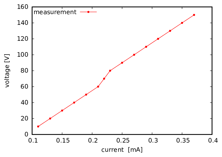
Jan, Yuri | Detectors | UI-diagram | 2021 | The UI-curve of the detector
U I
10 0.11
20 0.13
30 0.15
40 0.17
50 0.19
60 0.21
70 0.22
80 0.23
90 0.25
100 0.27
110 0.29
120 0.31
130 0.33
140 0.35
150 0.37 |
| Attachment 1: UI_meas_curve.pdf
|
|
|
291
|
Thu Apr 22 10:56:20 2021 |
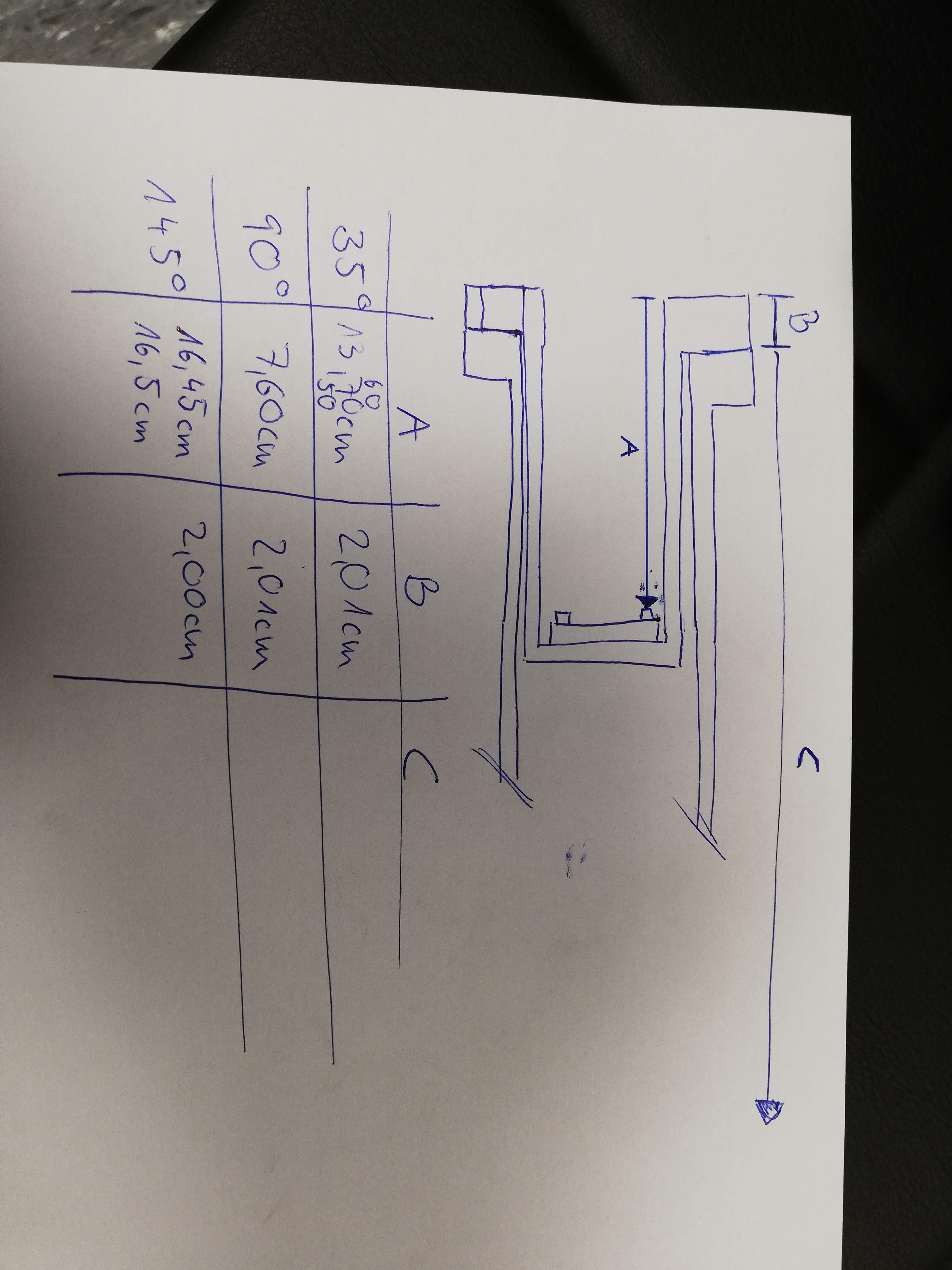
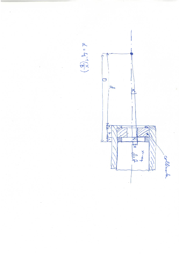
Jan | Detectors | target-chamber det. distances | 2021 | This is the lookup table for the distance of each x-ray detector to the target.
See attached foto for explanation.
It is the same values as in 2020: https://elog.gsi.de/esr/E127/36
|
Detector | A (dA) [mm] | B (dB) [mm] | C (dC) [mm] | calculate | result [mm]
| |
35° | 136.0 (1.0) | 20.0 (0.2) | 450.0 (0.5) | C + B - A | 334.0 (?)
| |
90° | 76.0 (0.5) | 20.0 (0.2) | 447.0/2 = 223.5 (1.0) | C + B - A | 167.5 (?)
| |
145° | 165.0 (1.0) | 20.0 (0.2) | 450.0 (0.5) | C + B - A | 305.0 (?)
|
Errors are estimated after measurement, final errorbars have to be double checked! |
| Attachment 1: E127_xray_distances.jpg
|
|
|
290
|
Wed Apr 14 09:42:50 2021 |
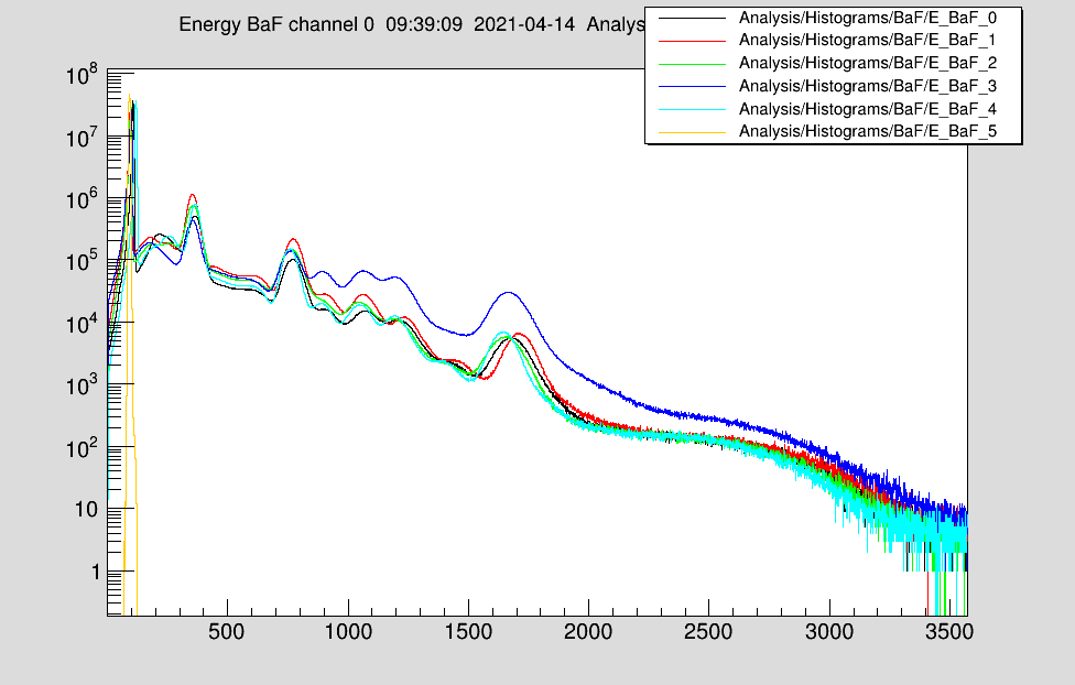
Jan | Detectors | BaF HV gain matching | 2021 | The preliminary gain matching settings for a full ADC range of ~12MeV:
|
Det.Nr. | ADC/TDC ch | HV | I | comment
| |
1 | 20 | 2400V | 390uA | CAEN HV ch0
| |
2 | 21 | 1763V | 287uA | CAEN HV ch1
| |
3 | 22 | 2340V | 380uA | CAEN HV ch2
| |
4 | 23 | 2175V | 354uA | CAEN HV ch3
| |
5 | 24 | 2017.5V | ? | emetron HV
| |
6 | 25 | 1780V | ? | not yet biased
|
Attached is a 22Na-spectrum taken with detectors 1 - 5.
The used MSCF settings are also attached.
Detector 6 does not yet have a HV channel available. |
| Attachment 1: BaF_Na22_gain_match_v1.png
|
|
| Attachment 2: baf_gain_match_v1.dat
|
atpnuc006:mrcc:mscf1:getGainCommon 15
atpnuc006:mrcc:mscf1:getShapingTimeCommon 3
atpnuc006:mrcc:mscf1:getThresholdCommon 6
atpnuc006:mrcc:mscf1:getPzCommon 6
atpnuc006:mrcc:mscf1:getGain1  6
atpnuc006:mrcc:mscf1:getGain2  6
atpnuc006:mrcc:mscf1:getGain3  6
atpnuc006:mrcc:mscf1:getGain4  6
atpnuc006:mrcc:mscf1:getShapingTime1 3
atpnuc006:mrcc:mscf1:getShapingTime2 3
atpnuc006:mrcc:mscf1:getShapingTime3 3
atpnuc006:mrcc:mscf1:getShapingTime4 3
atpnuc006:mrcc:mscf1:getThreshold1 6
atpnuc006:mrcc:mscf1:getThreshold2 6
atpnuc006:mrcc:mscf1:getThreshold3 6
atpnuc006:mrcc:mscf1:getThreshold4 6
atpnuc006:mrcc:mscf1:getThreshold5 6
atpnuc006:mrcc:mscf1:getThreshold6 6
atpnuc006:mrcc:mscf1:getThreshold7 6
atpnuc006:mrcc:mscf1:getThreshold8 6
atpnuc006:mrcc:mscf1:getThreshold9 6
atpnuc006:mrcc:mscf1:getThreshold10 6
atpnuc006:mrcc:mscf1:getThreshold11 6
atpnuc006:mrcc:mscf1:getThreshold12 6
atpnuc006:mrcc:mscf1:getThreshold13 6
atpnuc006:mrcc:mscf1:getThreshold14 6
atpnuc006:mrcc:mscf1:getThreshold15 6
atpnuc006:mrcc:mscf1:getThreshold16 6
atpnuc006:mrcc:mscf1:getPz1    6
atpnuc006:mrcc:mscf1:getPz2    3
atpnuc006:mrcc:mscf1:getPz3    3
atpnuc006:mrcc:mscf1:getPz4    1
atpnuc006:mrcc:mscf1:getPz5    5
atpnuc006:mrcc:mscf1:getPz6    5
atpnuc006:mrcc:mscf1:getPz7    6
atpnuc006:mrcc:mscf1:getPz8    6
atpnuc006:mrcc:mscf1:getPz9    6
atpnuc006:mrcc:mscf1:getPz10   6
atpnuc006:mrcc:mscf1:getPz11   6
atpnuc006:mrcc:mscf1:getPz12   6
atpnuc006:mrcc:mscf1:getPz13   6
atpnuc006:mrcc:mscf1:getPz14   6
atpnuc006:mrcc:mscf1:getPz15   6
atpnuc006:mrcc:mscf1:getPz16   6
atpnuc006:mrcc:mscf1:getSingleChMode 1
atpnuc006:mrcc:mscf1:getRcMode 1
atpnuc006:mrcc:mscf1:getAutoPZ 0
atpnuc006:mrcc:mscf1:getMultiplicityHi 8
atpnuc006:mrcc:mscf1:getMultiplicityLo 1
atpnuc006:mrcc:mscf1:getSumTrgThresh 100
atpnuc006:mrcc:mscf1:getBlrOn  0
atpnuc006:mrcc:mscf1:getCoincTime 100
atpnuc006:mrcc:mscf1:getThreshOffset 1
atpnuc006:mrcc:mscf1:getShaperOffset 100
atpnuc006:mrcc:mscf1:getBlrThresh 10
atpnuc006:mrcc:mscf1:getECLDelay 0
|
|
289
|
Wed Mar 31 13:57:27 2021 |
Jan | Detectors | BaF HV settings | 2021 | The setting below is a start value for final gain matching with a full ADC range of 12MeV:
|
Det.Nr. | ADC/TDC ch | HV | MSCF Gain
| |
1 | 20 | 2400V | 6
| |
2 | 21 | 1780V | 6
| |
3 | 22 | 2350V | 6
| |
4 | 23 | 2130V | 6
| |
5 | 24 | 2050V | 6
| |
6 | 25 | 1780V | 6
|
|
|
288
|
Wed Mar 31 13:52:04 2021 |
Jan | Detectors | BaF Na22 Testing | 2021 | On 30. and 31.03.2021 we did some testing with the 6 BaF detectors.
Trigger & threshold:
With a threshold at ~250 keV, each detector has an trigger rate of about 0.5kHz due to internal activity.
Energy spectra
All detectors showed the Na22 lines (511 + 1275 keV) and also the lines from internal activity.
The energy resolution was on the order of 8.5 - 11 keV, depending on the detector.
Time spectra
Raw TDC spectra showed self-stop peak.
TDC diff spectra (between detectors) show one main (sharp) correlation peak about 8ns = 30ch*0.293ns/ch off the zero.
At very low intensity a time structure around this peak is visible in a region of 120ns around the main peak. This is not understood, the energy spectra look similar for all these time regions (above/on/below the main peak).
Additionally, the coincidence E-specta between detector 1 and 2 (gating on the main time peak), nicely showed only the 511 keV line from Na22 and some gras.
Overnight test run:
Det. 1, 2, 3, 4 with the Na22 source
lxg1275:/data.local3/e127/lmd_2021/test/
e127b_run0021.lmd
e127b_run0022.lmd
e127b_run0023.lmd
e127b_run0024.lmd
e127b_run0025.lmd
e127b_run0026.lmd
e127b_run0027.lmd
e127b_run0028.lmd
e127b_run0029.lmd
e127b_run0030.lmd
e127b_run0031.lmd
e127b_run0032.lmd
e127b_run0033.lmd
e127b_run0034.lmd
Gain matched HV settings: https://elog.gsi.de/esr/E127/289
Issues to solve:
- 2 missing HV channels
- Go4 Analysis not stable
- trigger not on Baf but on Si |
|
287
|
Tue Feb 2 13:59:00 2021 |
Jan | Detectors | DSSD installation and alignment | 2021 | The DSSD has been exchanged and aligned in
November 2020. After bakeout at 140°C
(externally, 120°C at internal temp. Sensor)
for more than a week, the vacuum in the setup
is roughly 4.5e-10 mbar.
After the bakeout the detector had to be
realigned, it was lower by 1-2 mm. Using the
line laser the realignment was done by
touching only the screws on the far part of
the base of the flange. These screws have been
thightend by about a 1/4 turn after releasing
the headless positioning screw accordingly. |
|
286
|
Tue Nov 24 15:35:49 2020 |
Jan | Calibration | DSSD X/Y channel mapping | 2021 | During the detector test test measurements with alpha source the allocation of the 16 X- and 16 Y-channels has been checked.
For the following final allocation, it is always assumed that the (horizontal) y-strips are placed to face the beam directly, while the (vertical) x-strips are on the backside.
Now, all cables from the preamp to the ADC/TDCs are either labeled BLACK (= X-strips, pos. signals) or labeled RED (= Y-strips, neg. signals). These red or black connections should be kept consistently in order to ensure a well known orientation of the DSSD during the experiment. The test run Si2_run006.lmd was taken with this final assignment and serves as reference.
BLACK LABEL > X1 to X16 > pos. MSCF > ADC/TDC ch 0-15 > 50 Ohm resistor at preamps HV-input
RED LABEL > Y1 to Y16 > neg. MSCF > ADC/TDC ch 16-31 > neg. bias voltage at preamps HV-input
Additionally, the RED label indicates the section on the preamp to which negative bias voltage should be applied. |
|
285
|
Fri Nov 20 15:53:37 2020 |
Jan | Analysis | Test of 2nd DSSSD (gen2) | 2021 | Here is the analysis of the test runs with the 2nd DSSD (gen2) using the quick_si_plots.c script attached.
All 32 Si channels are working with acceptable performance.
In run001, there are some additional low energy peaks in nearly all x-strips, which I do not understand yet. They are around 3 MeV and are not visible in the y-strips. It doesn't look like an electronic problem, because there are at least 4
peaks, so not a low amplitude copy of the 3 major alpha peaks between 5 - 5.8 MeV.
However, in run002, the peaks have mostly disappeared, only in x6,x7,x8,x9 is a broad structure at somewhat similar energy... maybe this has to do with the small incident angle of the alphas?
Another run to confirm and double check this would be nice. |
| Attachment 1: quick_si_plots.c
|
//Created by Laszo Varga & Jan Glorius
//last update: 20.11.2020

//run in root:
//root -l
//.L script.c+
//run()
////////////////////////

// INPUT FILES
#define INPUT1 "/data.local3/test_data_2020/Si2_run002.lmd.root"

//OUTPUT FILE
#define OUTPUT "Si2_run002.ana.root"

//Energy thresholds for the silicon:
#define Si_Thrs_LOW 100
#define Si_Thrs_HIGH 8000

////////////////////////

#include <cmath>
#include <string>
#include <cstdlib>
#include <cstdio>
#include <ctime>
#include <fstream>
#include <iostream>
#include <stdint.h>
#include "TROOT.h"
#include "TAttText.h"
#include "TAxis.h"
#include "TCanvas.h"
#include "TChain.h"
#include "TCut.h"
#include "TF1.h"
#include "TFile.h"
#include "TGraph.h"
#include "TGraphAsymmErrors.h"
#include "TGraphErrors.h"
#include "TH1.h"
#include "TH2.h"
#include "THistPainter.h"
#include "TKey.h"
#include "TLatex.h"
#include "TLegend.h"
#include "TMath.h"
#include "TMatrixD.h"
#include "TMinuit.h"
#include "TMultiGraph.h"
#include "TNtuple.h"
#include "TPave.h"
#include "TPaveText.h"
#include "TPoint.h"
#include "TRandom.h"
#include "TRint.h"
#include "TStyle.h"
#include "TString.h"
#include "TTree.h"
#include "TH1F.h"
#include "TH2F.h"
#include "TSystem.h"
#include "TProfile.h"
#include "TVirtualFitter.h"
#include "TCanvas.h"
#include "TLegend.h"
#include "TColor.h"

using namespace std;

void loop(TChain *fChain){

#include "/data.local3/test_data_2020/e127.h"

//creating histos

//counting of variables starts from 0 --> eg.: first Si strip is 0.

TH2D *h_pos_Si_xy_raw=new TH2D("h_pos_si_xy_raw", "h_pos_si_xy_raw",16,-0.5,15.5,16,-0.5,15.5);
TH2D *h_pos_Si_xy_noDC=new TH2D("h_pos_si_xy_noDC", "h_pos_si_xy_noDC",16,-0.5,15.5,16,-0.5,15.5);

TH2D *h_E_Si_all=new TH2D("h_E_Si_all", "E vs. strip Nr.; strip nr.; energy ",32,-0.5,31.5,8192,0.5,8191.5);

TH1D *h_E_Si_x[16];
TH1D *h_E_Si_y[16];
TH2D *h_E_ev_x[16];
TH2D *h_E_ev_y[16];

for(int a=0;a<16;a++){
	h_E_Si_x[a]=new TH1D(Form("h_E_Si_x%d",a),Form("h_E_Si_x%d",a),8192,0.5,8191.5);
	h_E_Si_y[a]=new TH1D(Form("h_E_Si_y%d",a),Form("h_E_Si_y%d",a),8192,0.5,8191.5);
	h_E_ev_x[a]=new TH2D(Form("h_E_ev_x%d",a),Form("h_E_ev_x%d;ev;E",a),1024,0,55e6,4096,0.5,8191.5);
	h_E_ev_y[a]=new TH2D(Form("h_E_ev_y%d",a),Form("h_E_ev_y%d;ev;E",a),1024,0,55e6,4096,0.5,8191.5);
}

////////////////////////////////////////////////////////////////////////

Long64_t nentries = fChain->GetEntries();
Long64_t nbytes = 0;

int dc_y_max=-999;
int dc_x_max=-999;
int dc_Ey_max=0;
int dc_Ex_max=0;
int dc_ty_max=0;
int dc_tx_max=0;

for (Long64_t i=0; i<nentries;i++){
//for (Long64_t i=0; i<100000;i++){
  nbytes += fChain->GetEntry(i);
	// event countdown
	if ((float(i)/100000.)==int(i/100000)){cout << "event: " << i << " \tof " << nentries << endl;}

	if(trigger==1){

		for (int i_x=0;i_x<16;i_x++){
			for (int i_y=0;i_y<16;i_y++){

			  if(int(E_Si_x[i_x])> 2000 && int(E_Si_y[i_y])> 2000)
			    {
			      h_pos_Si_xy_raw->Fill(i_x,i_y);
			    }

			  if(int(E_Si_x[i_x])>dc_Ex_max && int(E_Si_y[i_y])>dc_Ey_max){
			    dc_y_max = i_y;
			    dc_x_max = i_x;
			    dc_Ey_max = E_Si_y[i_y];
			    dc_Ex_max = E_Si_x[i_x];
			    dc_ty_max = t_Si_y[i_y];
			    dc_tx_max = t_Si_x[i_x];
			  }
			}

			//x-loop is missused for y also
			if(t_Si_x[i_x] > 0){
			  h_E_Si_all->Fill(i_x,E_Si_x[i_x]);
			  h_E_Si_x[i_x]->Fill(E_Si_x[i_x]);
			}
			if(t_Si_y[i_x] > 0){
			  h_E_Si_all->Fill(i_x + 16,E_Si_y[i_x]);
			  h_E_Si_y[i_x]->Fill(E_Si_y[i_x]);
			}


		}

		if(dc_x_max!=-999 && dc_y_max!=-999){
			h_pos_Si_xy_noDC->Fill(dc_x_max,dc_y_max);
			h_E_ev_x[dc_x_max]->Fill(i,dc_Ex_max);
			h_E_ev_y[dc_y_max]->Fill(i,dc_Ey_max);
		}

		dc_y_max=-999;
		dc_x_max=-999;
		dc_Ex_max=0;
		dc_Ey_max=0;
		dc_tx_max=0;
		dc_ty_max=0;
	}
 }//event loop

 TFile *graphfile = TFile::Open(OUTPUT, "RECREATE");

//graphfile->mkdir("Si_map");
//graphfile->cd("Si_map");
 h_pos_Si_xy_raw->Write();
 h_pos_Si_xy_noDC->Write();
 h_E_Si_all->Write();

//graphfile->mkdir("Si_E_histos");
//graphfile->cd("Si_E_histos");
 for(int a=0;a<16;a++){
   h_E_Si_x[a]->Write();
   h_E_Si_y[a]->Write();
   h_E_ev_x[a]->Write();
   h_E_ev_y[a]->Write();
 }

graphfile->Close();
cout << "\033[0;32m" << OUTPUT << " is created!\033[0m" << endl;

} // loop

void run(){

  const char    *command = new char[1000];
  char filename[100];
  TChain *fChain = new TChain("h101");

  sprintf(filename,INPUT1);
  cout<<"\033[0;37m//loading run: "<<filename << "\033[0m" <<endl;
  fChain->Add(filename);

#ifdef INPUT2 // optional second input file
  sprintf(filename,INPUT2);
  cout<<"\033[0;37m//loading run: "<<filename << "\033[0m" <<endl;
  fChain->Add(filename);
#endif

//sprintf(filename,OUTPUT);
//	TFile *outfile = new TFile(filename,"RECREATE");

  loop(fChain);

//  outfile->Write();

  command = "rm  *.so";
  gSystem->Exec(command);
  command = "rm  *.d";
  gSystem->Exec(command);
  command = "rm  *.pcm";
  gSystem->Exec(command);

  return;
}

int main(){
 run();

  return(0);
}
|
| Attachment 2: e127.h
|
//Declaration of leaves types
UInt_t tpat;
UInt_t trigger;
UInt_t Si_voltage;
UInt_t Si_current;
UInt_t E_Si_y[16];
UInt_t E_Si_x[16];
UInt_t E_Xray[3];
UInt_t E_BaF[6];
UInt_t t_Si_y[16];
UInt_t t_Si_x[16];
UInt_t t_Xray[3];
UInt_t t_BaF[6];
UInt_t v_mega_clock;
UInt_t v_Si_X;
UInt_t v_Si_Y;
UInt_t v_Xray[3];
UInt_t v_BaF[6];
UInt_t v_TRAFO;
UInt_t v_I_cool;
UInt_t v_U_cool;
UInt_t v_jet_S[1];
UInt_t bdt_si_ON;
UInt_t bdt_si_OFF;
UInt_t bdt_xray_ON;
UInt_t bdt_xray_OFF;
UInt_t bdt_baf_ON;
UInt_t bdt_baf_OFF;
UInt_t adt_si_ON;
UInt_t adt_si_OFF;
UInt_t adt_xray_ON;
UInt_t adt_xray_OFF;
UInt_t adt_baf_ON;
UInt_t adt_baf_OFF;
UInt_t red_si_ON;
UInt_t red_si_OFF;
UInt_t red_xray_ON;
UInt_t red_xray_OFF;
UInt_t red_baf_ON;
UInt_t red_baf_OFF;
// Set branch addresses.
fChain->SetBranchAddress("tpat",&tpat);
fChain->SetBranchAddress("TRIGGER",&trigger);
fChain->SetBranchAddress("Si_voltage",&Si_voltage);
fChain->SetBranchAddress("Si_current",&Si_current);
fChain->SetBranchAddress("E_Si_y1",&E_Si_y[0]);
fChain->SetBranchAddress("E_Si_y2",&E_Si_y[1]);
fChain->SetBranchAddress("E_Si_y3",&E_Si_y[2]);
fChain->SetBranchAddress("E_Si_y4",&E_Si_y[3]);
fChain->SetBranchAddress("E_Si_y5",&E_Si_y[4]);
fChain->SetBranchAddress("E_Si_y6",&E_Si_y[5]);
fChain->SetBranchAddress("E_Si_y7",&E_Si_y[6]);
fChain->SetBranchAddress("E_Si_y8",&E_Si_y[7]);
fChain->SetBranchAddress("E_Si_y9",&E_Si_y[8]);
fChain->SetBranchAddress("E_Si_y10",&E_Si_y[9]);
fChain->SetBranchAddress("E_Si_y11",&E_Si_y[10]);
fChain->SetBranchAddress("E_Si_y12",&E_Si_y[11]);
fChain->SetBranchAddress("E_Si_y13",&E_Si_y[12]);
fChain->SetBranchAddress("E_Si_y14",&E_Si_y[13]);
fChain->SetBranchAddress("E_Si_y15",&E_Si_y[14]);
fChain->SetBranchAddress("E_Si_y16",&E_Si_y[15]);
fChain->SetBranchAddress("E_Si_x1",&E_Si_x[0]);
fChain->SetBranchAddress("E_Si_x2",&E_Si_x[1]);
fChain->SetBranchAddress("E_Si_x3",&E_Si_x[2]);
fChain->SetBranchAddress("E_Si_x4",&E_Si_x[3]);
fChain->SetBranchAddress("E_Si_x5",&E_Si_x[4]);
fChain->SetBranchAddress("E_Si_x6",&E_Si_x[5]);
fChain->SetBranchAddress("E_Si_x7",&E_Si_x[6]);
fChain->SetBranchAddress("E_Si_x8",&E_Si_x[7]);
fChain->SetBranchAddress("E_Si_x9",&E_Si_x[8]);
fChain->SetBranchAddress("E_Si_x10",&E_Si_x[9]);
fChain->SetBranchAddress("E_Si_x11",&E_Si_x[10]);
fChain->SetBranchAddress("E_Si_x12",&E_Si_x[11]);
fChain->SetBranchAddress("E_Si_x13",&E_Si_x[12]);
fChain->SetBranchAddress("E_Si_x14",&E_Si_x[13]);
fChain->SetBranchAddress("E_Si_x15",&E_Si_x[14]);
fChain->SetBranchAddress("E_Si_x16",&E_Si_x[15]);
fChain->SetBranchAddress("E_Xray1",&E_Xray[0]);
fChain->SetBranchAddress("E_Xray2",&E_Xray[1]);
fChain->SetBranchAddress("E_Xray3",&E_Xray[2]);
fChain->SetBranchAddress("E_BaF1",&E_BaF[0]);
fChain->SetBranchAddress("E_BaF2",&E_BaF[1]);
fChain->SetBranchAddress("E_BaF3",&E_BaF[2]);
fChain->SetBranchAddress("E_BaF4",&E_BaF[3]);
fChain->SetBranchAddress("E_BaF5",&E_BaF[4]);
fChain->SetBranchAddress("E_BaF6",&E_BaF[5]);
fChain->SetBranchAddress("t_Si_y1",&t_Si_y[0]);
fChain->SetBranchAddress("t_Si_y2",&t_Si_y[1]);
fChain->SetBranchAddress("t_Si_y3",&t_Si_y[2]);
fChain->SetBranchAddress("t_Si_y4",&t_Si_y[3]);
fChain->SetBranchAddress("t_Si_y5",&t_Si_y[4]);
fChain->SetBranchAddress("t_Si_y6",&t_Si_y[5]);
fChain->SetBranchAddress("t_Si_y7",&t_Si_y[6]);
fChain->SetBranchAddress("t_Si_y8",&t_Si_y[7]);
fChain->SetBranchAddress("t_Si_y9",&t_Si_y[8]);
fChain->SetBranchAddress("t_Si_y10",&t_Si_y[9]);
fChain->SetBranchAddress("t_Si_y11",&t_Si_y[10]);
fChain->SetBranchAddress("t_Si_y12",&t_Si_y[11]);
fChain->SetBranchAddress("t_Si_y13",&t_Si_y[12]);
fChain->SetBranchAddress("t_Si_y14",&t_Si_y[13]);
fChain->SetBranchAddress("t_Si_y15",&t_Si_y[14]);
fChain->SetBranchAddress("t_Si_y16",&t_Si_y[15]);
fChain->SetBranchAddress("t_Si_x1",&t_Si_x[0]);
fChain->SetBranchAddress("t_Si_x2",&t_Si_x[1]);
fChain->SetBranchAddress("t_Si_x3",&t_Si_x[2]);
fChain->SetBranchAddress("t_Si_x4",&t_Si_x[3]);
fChain->SetBranchAddress("t_Si_x5",&t_Si_x[4]);
fChain->SetBranchAddress("t_Si_x6",&t_Si_x[5]);
fChain->SetBranchAddress("t_Si_x7",&t_Si_x[6]);
fChain->SetBranchAddress("t_Si_x8",&t_Si_x[7]);
fChain->SetBranchAddress("t_Si_x9",&t_Si_x[8]);
fChain->SetBranchAddress("t_Si_x10",&t_Si_x[9]);
fChain->SetBranchAddress("t_Si_x11",&t_Si_x[10]);
fChain->SetBranchAddress("t_Si_x12",&t_Si_x[11]);
fChain->SetBranchAddress("t_Si_x13",&t_Si_x[12]);
fChain->SetBranchAddress("t_Si_x14",&t_Si_x[13]);
fChain->SetBranchAddress("t_Si_x15",&t_Si_x[14]);
fChain->SetBranchAddress("t_Si_x16",&t_Si_x[15]);
fChain->SetBranchAddress("t_Xray1",&t_Xray[0]);
fChain->SetBranchAddress("t_Xray2",&t_Xray[1]);
fChain->SetBranchAddress("t_Xray3",&t_Xray[2]);
fChain->SetBranchAddress("t_BaF1",&t_BaF[0]);
fChain->SetBranchAddress("t_BaF2",&t_BaF[1]);
fChain->SetBranchAddress("t_BaF3",&t_BaF[2]);
fChain->SetBranchAddress("t_BaF4",&t_BaF[3]);
fChain->SetBranchAddress("t_BaF5",&t_BaF[4]);
fChain->SetBranchAddress("t_BaF6",&t_BaF[5]);
fChain->SetBranchAddress("v_mega_clock",&v_mega_clock);
fChain->SetBranchAddress("v_Si_X",&v_Si_X);
fChain->SetBranchAddress("v_Si_Y",&v_Si_Y);
fChain->SetBranchAddress("v_Xray1",&v_Xray[0]);
fChain->SetBranchAddress("v_Xray2",&v_Xray[1]);
fChain->SetBranchAddress("v_Xray3",&v_Xray[2]);
fChain->SetBranchAddress("v_BaF1",&v_BaF[0]);
fChain->SetBranchAddress("v_BaF2",&v_BaF[1]);
fChain->SetBranchAddress("v_BaF3",&v_BaF[2]);
fChain->SetBranchAddress("v_BaF4",&v_BaF[3]);
fChain->SetBranchAddress("v_BaF5",&v_BaF[4]);
fChain->SetBranchAddress("v_BaF6",&v_BaF[5]);
fChain->SetBranchAddress("v_TRAFO",&v_TRAFO);
fChain->SetBranchAddress("v_I_cool",&v_I_cool);
fChain->SetBranchAddress("v_U_cool",&v_U_cool);
fChain->SetBranchAddress("v_jet_S1",&v_jet_S[0]);
fChain->SetBranchAddress("bdt_si_ON",&bdt_si_ON);
fChain->SetBranchAddress("bdt_si_OFF",&bdt_si_OFF);
fChain->SetBranchAddress("bdt_xray_ON",&bdt_xray_ON);
fChain->SetBranchAddress("bdt_xray_OFF",&bdt_xray_OFF);
fChain->SetBranchAddress("bdt_baf_ON",&bdt_baf_ON);
fChain->SetBranchAddress("bdt_baf_OFF",&bdt_baf_OFF);
fChain->SetBranchAddress("adt_si_ON",&adt_si_ON);
fChain->SetBranchAddress("adt_si_OFF",&adt_si_OFF);
fChain->SetBranchAddress("adt_xray_ON",&adt_xray_ON);
fChain->SetBranchAddress("adt_xray_OFF",&adt_xray_OFF);
fChain->SetBranchAddress("adt_baf_ON",&adt_baf_ON);
fChain->SetBranchAddress("adt_baf_OFF",&adt_baf_OFF);
fChain->SetBranchAddress("red_si_ON",&red_si_ON);
fChain->SetBranchAddress("red_si_OFF",&red_si_OFF);
fChain->SetBranchAddress("red_xray_ON",&red_xray_ON);
fChain->SetBranchAddress("red_xray_OFF",&red_xray_OFF);
fChain->SetBranchAddress("red_baf_ON",&red_baf_ON);
fChain->SetBranchAddress("red_baf_OFF",&red_baf_OFF);
/*
fChain->SetBranchAddress("tpat",&tpat);
fChain->SetBranchAddress("trigger",&trigger);
fChain->SetBranchAddress("timestamp_lsb",×tamp_lsb);
fChain->SetBranchAddress("timestamp_msb",×tamp_msb);
fChain->SetBranchAddress("Tsc_before_lmu1",&Tsc_before_lmu[1]);
fChain->SetBranchAddress("Tsc_before_lmu1",&Tsc_before_lmu1);
fChain->SetBranchAddress("Tsc_before_lmu2",&Tsc_before_lmu2);
fChain->SetBranchAddress("Tsc_before_lmu3",&Tsc_before_lmu3);
fChain->SetBranchAddress("Tsc_before_lmu4",&Tsc_before_lmu4);
fChain->SetBranchAddress("Tsc_before_lmu5",&Tsc_before_lmu5);
fChain->SetBranchAddress("Tsc_before_lmu6",&Tsc_before_lmu6);
fChain->SetBranchAddress("Tsc_before_lmu7",&Tsc_before_lmu7);
fChain->SetBranchAddress("Tsc_before_lmu8",&Tsc_before_lmu8);
fChain->SetBranchAddress("Tsc_before_lmu9",&Tsc_before_lmu9);
fChain->SetBranchAddress("Tsc_before_lmu10",&Tsc_before_lmu10);
fChain->SetBranchAddress("Tsc_before_lmu11",&Tsc_before_lmu11);
fChain->SetBranchAddress("Tsc_before_lmu12",&Tsc_before_lmu12);
fChain->SetBranchAddress("Tsc_before_lmu13",&Tsc_before_lmu13);
fChain->SetBranchAddress("Tsc_before_lmu14",&Tsc_before_lmu14);
fChain->SetBranchAddress("Tsc_before_lmu15",&Tsc_before_lmu15);
fChain->SetBranchAddress("Tsc_before_lmu16",&Tsc_before_lmu16);
fChain->SetBranchAddress("Tsc_before_dt1",&Tsc_before_dt1);
fChain->SetBranchAddress("Tsc_before_dt2",&Tsc_before_dt2);
fChain->SetBranchAddress("Tsc_before_dt3",&Tsc_before_dt3);
fChain->SetBranchAddress("Tsc_before_dt4",&Tsc_before_dt4);
fChain->SetBranchAddress("Tsc_before_dt5",&Tsc_before_dt5);
fChain->SetBranchAddress("Tsc_before_dt6",&Tsc_before_dt6);
fChain->SetBranchAddress("Tsc_before_dt7",&Tsc_before_dt7);
fChain->SetBranchAddress("Tsc_before_dt8",&Tsc_before_dt8);
fChain->SetBranchAddress("Tsc_before_dt9",&Tsc_before_dt9);
fChain->SetBranchAddress("Tsc_before_dt10",&Tsc_before_dt10);
fChain->SetBranchAddress("Tsc_before_dt11",&Tsc_before_dt11);
fChain->SetBranchAddress("Tsc_before_dt12",&Tsc_before_dt12);
fChain->SetBranchAddress("Tsc_before_dt13",&Tsc_before_dt13);
fChain->SetBranchAddress("Tsc_before_dt14",&Tsc_before_dt14);
fChain->SetBranchAddress("Tsc_before_dt15",&Tsc_before_dt15);
fChain->SetBranchAddress("Tsc_before_dt16",&Tsc_before_dt16);
fChain->SetBranchAddress("Tsc_after_dt1",&Tsc_after_dt1);
fChain->SetBranchAddress("Tsc_after_dt2",&Tsc_after_dt2);
fChain->SetBranchAddress("Tsc_after_dt3",&Tsc_after_dt3);
fChain->SetBranchAddress("Tsc_after_dt4",&Tsc_after_dt4);
fChain->SetBranchAddress("Tsc_after_dt5",&Tsc_after_dt5);
fChain->SetBranchAddress("Tsc_after_dt6",&Tsc_after_dt6);
fChain->SetBranchAddress("Tsc_after_dt7",&Tsc_after_dt7);
fChain->SetBranchAddress("Tsc_after_dt8",&Tsc_after_dt8);
fChain->SetBranchAddress("Tsc_after_dt9",&Tsc_after_dt9);
fChain->SetBranchAddress("Tsc_after_dt10",&Tsc_after_dt10);
fChain->SetBranchAddress("Tsc_after_dt11",&Tsc_after_dt11);
fChain->SetBranchAddress("Tsc_after_dt12",&Tsc_after_dt12);
fChain->SetBranchAddress("Tsc_after_dt13",&Tsc_after_dt13);
fChain->SetBranchAddress("Tsc_after_dt14",&Tsc_after_dt14);
fChain->SetBranchAddress("Tsc_after_dt15",&Tsc_after_dt15);
fChain->SetBranchAddress("Tsc_after_dt16",&Tsc_after_dt16);
fChain->SetBranchAddress("E_Xray1",&E_Xray1);
fChain->SetBranchAddress("E_Xray2",&E_Xray2);
fChain->SetBranchAddress("E_Xray3",&E_Xray3);
fChain->SetBranchAddress("E_Xray4",&E_Xray4);
fChain->SetBranchAddress("E_Xray5",&E_Xray5);
fChain->SetBranchAddress("E_si_y1",&E_si_y[1]);
fChain->SetBranchAddress("E_si_y2",&E_si_y[2]);
fChain->SetBranchAddress("E_si_y3",&E_si_y[3]);
fChain->SetBranchAddress("E_si_y4",&E_si_y[4]);
fChain->SetBranchAddress("E_si_y5",&E_si_y[5]);
fChain->SetBranchAddress("E_si_y6",&E_si_y[6]);
fChain->SetBranchAddress("E_si_y7",&E_si_y[7]);
fChain->SetBranchAddress("E_si_y8",&E_si_y[8]);
fChain->SetBranchAddress("E_si_y9",&E_si_y[9]);
fChain->SetBranchAddress("E_si_y10",&E_si_y[10]);
fChain->SetBranchAddress("E_si_y11",&E_si_y[11]);
fChain->SetBranchAddress("E_si_y12",&E_si_y[12]);
fChain->SetBranchAddress("E_si_y13",&E_si_y[13]);
fChain->SetBranchAddress("E_si_y14",&E_si_y[14]);
fChain->SetBranchAddress("E_si_y15",&E_si_y[15]);
fChain->SetBranchAddress("E_si_y16",&E_si_y[16]);
fChain->SetBranchAddress("E_si_x1",&E_si_x[1]);
fChain->SetBranchAddress("E_si_x2",&E_si_x[2]);
fChain->SetBranchAddress("E_si_x3",&E_si_x[3]);
fChain->SetBranchAddress("E_si_x4",&E_si_x[4]);
fChain->SetBranchAddress("E_si_x5",&E_si_x[5]);
fChain->SetBranchAddress("E_si_x6",&E_si_x[6]);
fChain->SetBranchAddress("E_si_x7",&E_si_x[7]);
fChain->SetBranchAddress("E_si_x8",&E_si_x[8]);
fChain->SetBranchAddress("E_si_x9",&E_si_x[9]);
fChain->SetBranchAddress("E_si_x10",&E_si_x[10]);
fChain->SetBranchAddress("E_si_x11",&E_si_x[11]);
fChain->SetBranchAddress("E_si_x12",&E_si_x[12]);
fChain->SetBranchAddress("E_si_x13",&E_si_x[13]);
fChain->SetBranchAddress("E_si_x14",&E_si_x[14]);
fChain->SetBranchAddress("E_si_x15",&E_si_x[15]);
fChain->SetBranchAddress("E_si_x16",&E_si_x[16]);
fChain->SetBranchAddress("t_Xray1",&t_Xray1);
fChain->SetBranchAddress("t_Xray2",&t_Xray2);
fChain->SetBranchAddress("t_Xray3",&t_Xray3);
fChain->SetBranchAddress("t_Xray4",&t_Xray4);
fChain->SetBranchAddress("t_Xray5",&t_Xray5);
fChain->SetBranchAddress("t_MWPC_anode",&t_MWPC_anode);
fChain->SetBranchAddress("t_MWPC_x1",&t_MWPC_x1);
fChain->SetBranchAddress("t_MWPC_x2",&t_MWPC_x2);
fChain->SetBranchAddress("t_MWPC_y1",&t_MWPC_y1);
fChain->SetBranchAddress("t_MWPC_y2",&t_MWPC_y2);
fChain->SetBranchAddress("t_si_y1",&t_si_y[1]);
fChain->SetBranchAddress("t_si_y2",&t_si_y[2]);
fChain->SetBranchAddress("t_si_y3",&t_si_y[3]);
fChain->SetBranchAddress("t_si_y4",&t_si_y[4]);
fChain->SetBranchAddress("t_si_y5",&t_si_y[5]);
fChain->SetBranchAddress("t_si_y6",&t_si_y[6]);
fChain->SetBranchAddress("t_si_y7",&t_si_y[7]);
fChain->SetBranchAddress("t_si_y8",&t_si_y[8]);
fChain->SetBranchAddress("t_si_y9",&t_si_y[9]);
fChain->SetBranchAddress("t_si_y10",&t_si_y[10]);
fChain->SetBranchAddress("t_si_y11",&t_si_y[11]);
fChain->SetBranchAddress("t_si_y12",&t_si_y[12]);
fChain->SetBranchAddress("t_si_y13",&t_si_y[13]);
fChain->SetBranchAddress("t_si_y14",&t_si_y[14]);
fChain->SetBranchAddress("t_si_y15",&t_si_y[15]);
fChain->SetBranchAddress("t_si_y16",&t_si_y[16]);
fChain->SetBranchAddress("t_si_x1",&t_si_x[1]);
fChain->SetBranchAddress("t_si_x2",&t_si_x[2]);
fChain->SetBranchAddress("t_si_x3",&t_si_x[3]);
fChain->SetBranchAddress("t_si_x4",&t_si_x[4]);
fChain->SetBranchAddress("t_si_x5",&t_si_x[5]);
fChain->SetBranchAddress("t_si_x6",&t_si_x[6]);
fChain->SetBranchAddress("t_si_x7",&t_si_x[7]);
fChain->SetBranchAddress("t_si_x8",&t_si_x[8]);
fChain->SetBranchAddress("t_si_x9",&t_si_x[9]);
fChain->SetBranchAddress("t_si_x10",&t_si_x[10]);
fChain->SetBranchAddress("t_si_x11",&t_si_x[11]);
fChain->SetBranchAddress("t_si_x12",&t_si_x[12]);
fChain->SetBranchAddress("t_si_x13",&t_si_x[13]);
fChain->SetBranchAddress("t_si_x14",&t_si_x[14]);
fChain->SetBranchAddress("t_si_x15",&t_si_x[15]);
fChain->SetBranchAddress("t_si_x16",&t_si_x[16]);
fChain->SetBranchAddress("sc_TRIDI_clk",&sc[1]);
fChain->SetBranchAddress("sc_ext_clk",&sc[2]);
fChain->SetBranchAddress("SC3",&sc[3]);
fChain->SetBranchAddress("SC4",&sc[4]);
fChain->SetBranchAddress("SC5",&sc[5]);
fChain->SetBranchAddress("SC6",&sc[6]);
fChain->SetBranchAddress("SC7",&sc[7]);
fChain->SetBranchAddress("SC8",&sc[8]);
fChain->SetBranchAddress("sc_esr_trafo",&sc[9]);
fChain->SetBranchAddress("sc_I_cooler",&sc[10]);
fChain->SetBranchAddress("sc_U_cooler",&sc[11]);
fChain->SetBranchAddress("sc_jet_E1",&sc[12]);
fChain->SetBranchAddress("sc_jet_S1",&sc[13]);
fChain->SetBranchAddress("sc_jet_S2",&sc[14]);
fChain->SetBranchAddress("sc_jet_S3",&sc[15]);
fChain->SetBranchAddress("sc_jet_S4",&sc[16]);
fChain->SetBranchAddress("sc_si_y",&sc[17]);
fChain->SetBranchAddress("sc_si_x",&sc[18]);
fChain->SetBranchAddress("sc_xray1",&sc[19]);
fChain->SetBranchAddress("sc_xray2",&sc[20]);
fChain->SetBranchAddress("sc_xray3",&sc[21]);
fChain->SetBranchAddress("sc_xray4",&sc[22]);
fChain->SetBranchAddress("sc_mwpc",&sc[23]);
fChain->SetBranchAddress("sc_xray5",&sc[24]);
fChain->SetBranchAddress("sc_mwpcCFD",&sc[25]);
fChain->SetBranchAddress("SC26",&sc[26]);
fChain->SetBranchAddress("SC27",&sc[27]);
fChain->SetBranchAddress("SC28",&sc[28]);
fChain->SetBranchAddress("SC29",&sc[29]);
fChain->SetBranchAddress("SC30",&sc[30]);
fChain->SetBranchAddress("SC31",&sc[31]);
fChain->SetBranchAddress("SC32",&sc[32]);
*/
|
| Attachment 3: Si2_run001.ana.root
|
| Attachment 4: Si2_run002.ana.root
|
|
284
|
Fri Oct 23 12:58:12 2020 |
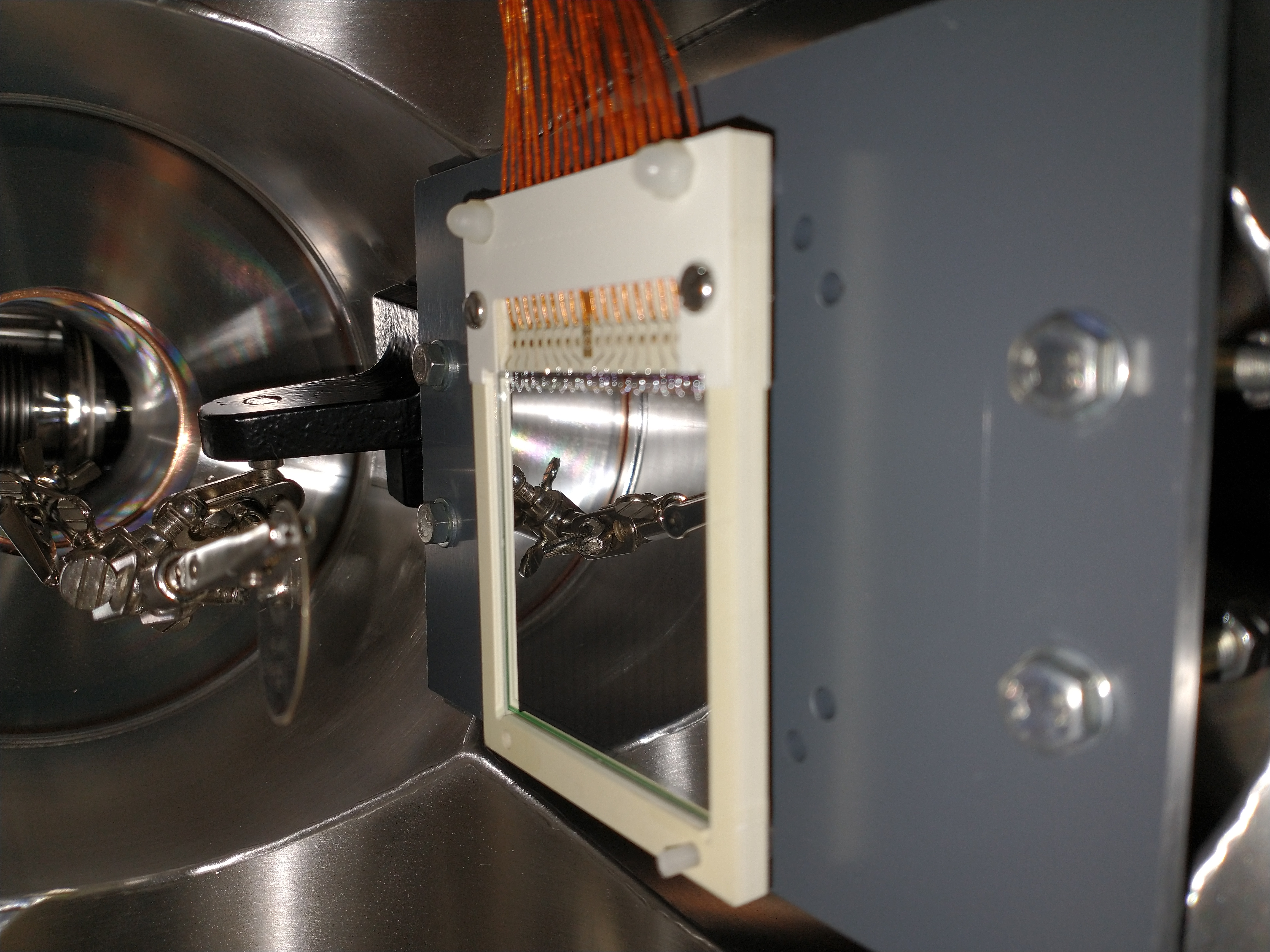
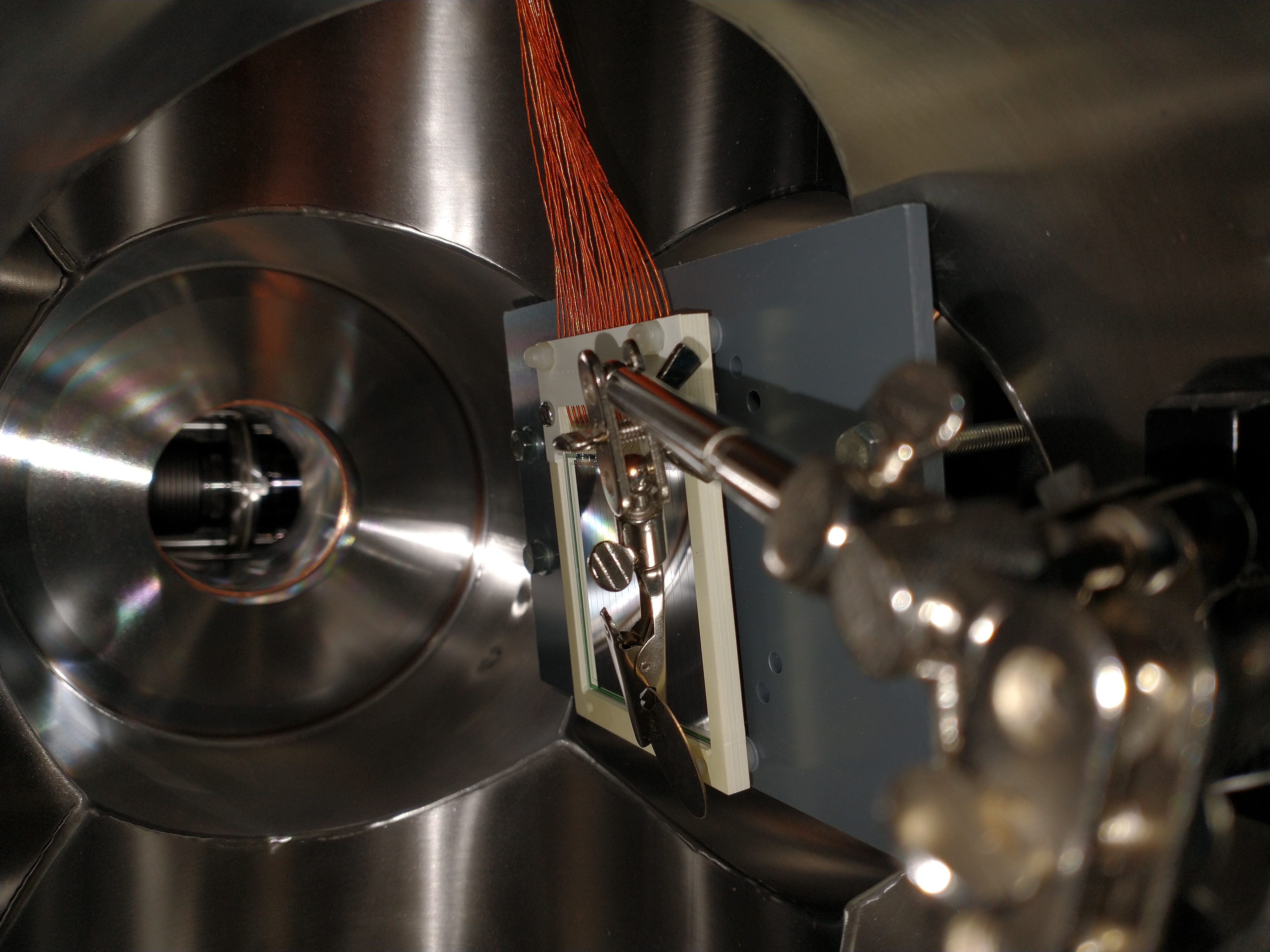
Jan | Detectors | Test of 2nd DSSSD (gen2) | 2021 | This is the documentation of the source tests with the 2nd micron DSSSD of 2nd generation (label 3288-17, thickness 529um)
The detector is put into vacuum (~5e-6 mbar) in our test chamber. The source is positioned a few cm above (see fotos).
The Bayard-Alpert Sensor in the chamber has to be deactivated, otherwise the light emission will increase the noise on the DSSSD strongly and reduce its performance.
Additionally the current and voltage from the CAEN HV is monitored with the vulom scalers: ch.13(Icool) = current; ch.14(Ucool) = voltage.
Source: mixes alpha [239Pu, 241Am, 244Cm]
File directory: lxg1275:/data.local3/test_data_2020/
QuickTest files: si2_test_mixed_source[X].root
lmd files: Si2_run[XXX].lmd
DAQ Settings:
MADC gate : 0 delay, 5000ns width
MSCF shaping: 2 us
trlo config : e127.trlo (trigger=1/tpat=1 for Si, trigger=11 for vulom_scaler)
LMD runs:
-----------------------------
Si2_run001.lmd
Start: Fri 23.10.2020 16:19
Stop: Mon 26.10.2020 8:36
File-Size: 20GB
Events: ~53M
comment:
source roughly centered
CAEN HV scalers not connected
-----------------------------
Si2_run002.lmd
Start: Tue 27.10.2020 16:01
Stop: Wed 28.10.2020 13:26
File-Size: 12GB
Events: ~32M
comment:
source in one corner (x1, y1, see foto)
scalers should be connected now
current monitor range set to LOW
@start det_current=140nA det_voltage=90V
@end det_current=143nA det_voltage=90V
-----------------------------
Si2_run003.lmd
Start: Wed 28.10.2020 13:30
Stop: Wed 28.10.2020 13:31
File-Size:
Events:
comment:
ramping of det. voltage for scaler/U-F-Converter test
source in one corner (see foto)
scalers should be connected now
current monitor range set to LOW
@start det_current=140nA det_voltage=90V
-----------------------------
Si2_run004.lmd
Start: Tue 24.11.2020 12:50
Stop: Tue 24.11.2020
File-Size:
Events:
comment:
source in one corner (x16, y16, see foto)
@start det_current=138nA det_voltage=90V
@end det_current=nA det_voltage=90V
-----------------------------
Si2_run005.lmd
Start: Tue 24.11.2020 14:57
Stop: Tue 24.11.2020 15:11
File-Size:
Events:
comment:
source in one corner (x1, y16, see foto)
@start det_current=144nA det_voltage=90V
@end det_current=nA det_voltage=90V
-----------------------------
Si2_run006.lmd
Start: Tue 24.11.2020 15:24
Stop: Tue 24.11.2020
File-Size:
Events:
comment:
source in one corner (x1, y16, see foto)
Si_X & Si_Y cabling to MADC_0 and TDC_0 exchanged to get right order of channels/orientation
@start det_current=144nA det_voltage=90V
@end det_current=nA det_voltage=90V |
| Attachment 1: Si2_run001.jpg
|
|
| Attachment 2: Si2_run002.jpg
|
|
|
283
|
Fri Jun 5 14:06:15 2020 |
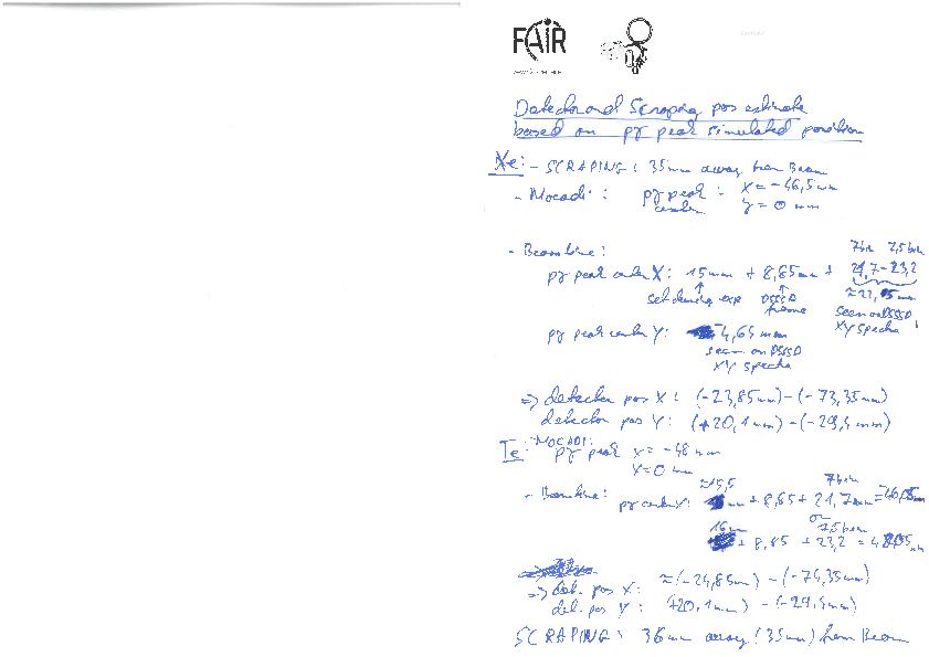
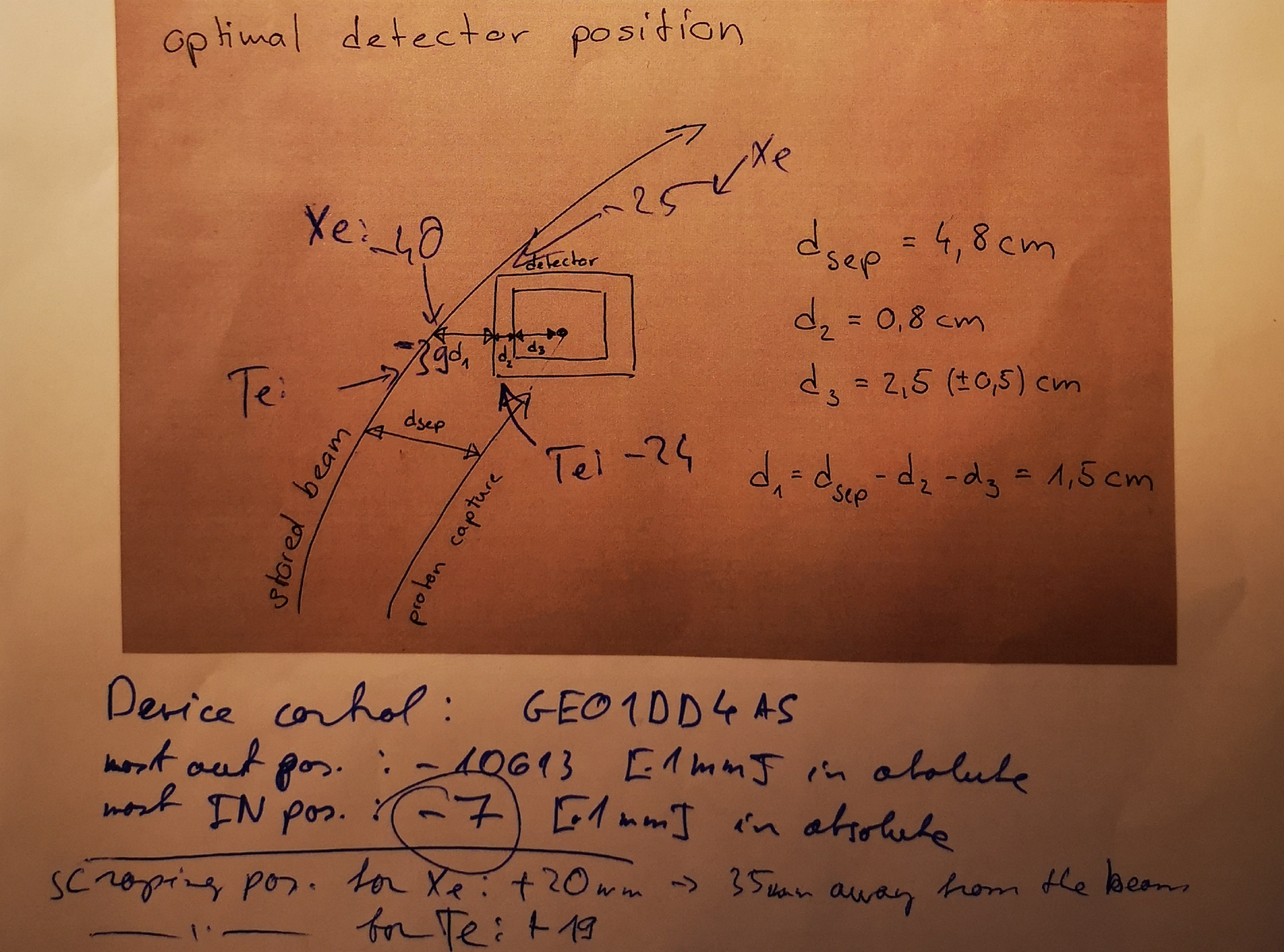
Laszlo | Detectors | DSSSD and SCRAPER position estimate for Xe and Te experiments | 2020 | We don't know the exact absolute positions of the detector (+scraper) and the beam. However, what we have to know is only these two relative positions respect to each other. To get this distance I use two methods:
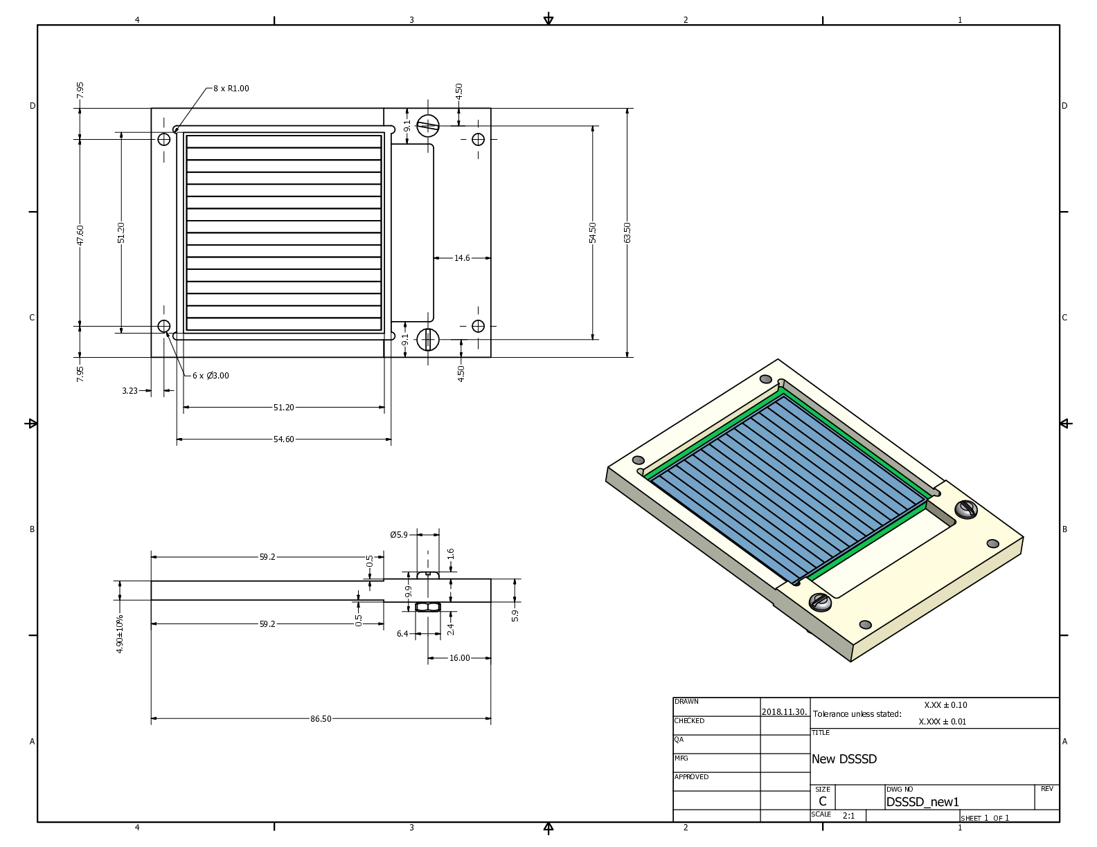
1, combining the infos from the set position during the beamtime + the measured pg peak position on the detector. The pg peak position is defined only by the eye (because of the low number of counts in every case, it doesnt make much sense to make fits). Since we rely on the detector resolution, we would be never more accurate than ~ +/-1.5mm anyhow. The active area of the detector is 49.5x49.5mm2 with a 45° tilt in y.
2, MOCADI simulation of the beam and the pg peak. This is used only as a crosscheck.
3, The scraper had a small angle in y direction causing ~0.5cm shift to the upper direction. the length of the scraping edge is 7cm
-124Xe with scraper measurement:
- measurement
d1 = moved back from beam = 15 +/-.5 mm
d2 = DSSSD frame width = 8.85 mm
d3 = pg center on DSSSD = 7-7.5 bin = 21.7-23.2 mm = avg = 22.5 mm
--> pg from beam in x = -46.4mm +/- 1.5mm
--> pg on DSSSD from center ~ -3.28mm +/- 1.5mm
- simulation
x = -46.5 mm
y = 0 mm
- detector active area position
x = (-73.35mm) - (-23.85mm)
y = (-14.2195mm) - 23.5125mm
- SCRAPING: x=-35mm +/-0.5mm away from beam
y=(-20mm) - (40mm)
-118Te:
- measurement
d1 = moved back from beam = 16 +/-.5 mm
d2 = DSSSD frame width = 8.85 mm
d3 = pg center on DSSSD = 7.5 bin = 23.2 mm
--> pg from beam in x = -48.05mm +/- 1.5mm
--> pg on DSSSD from center ~ -3.28mm +/- 1.5mm
- simulation
x = -48 mm
y = 0 mm
- detector active area position
x = (-74.35mm) - (-24.85mm)
y = (-14.2195mm) - 23.5125mm
- SCRAPING:
x=-35mm +/-0.5mm away from beam
y=(-20mm) - (40mm)
notes during beam-time:
https://elog.gsi.de/esr/E127/97?suppress=1 |
| Attachment 1: SP54120060514100.pdf
|
|
| Attachment 2: DSSSD_new1.pdf
|
|
| Attachment 3: IMG_20200321_025644.jpg
|
|
|
282
|
Tue May 19 16:48:15 2020 |
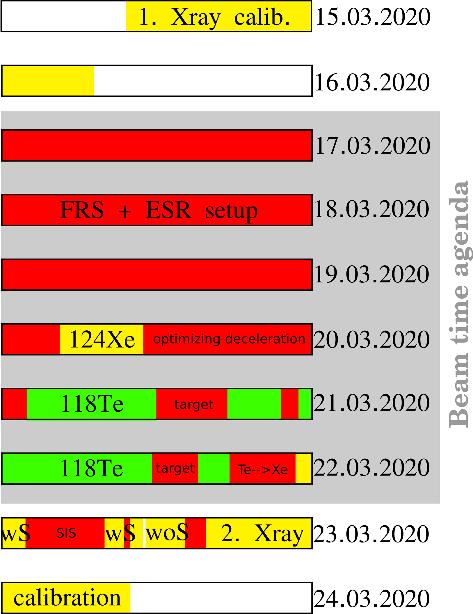
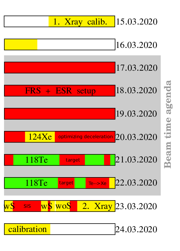
Laszlo | General | E127 beamtime overview | | Here is a representation how was the time management during E127. The time, what we could spend with measuring the 118Te(pg), was ~20% comparing to the given 6days. |
| Attachment 1: E127_beamtime_overview.png
|
|
| Attachment 2: E127_beamtime_overview.pdf
|
|
|
281
|
Wed May 6 23:02:42 2020 |
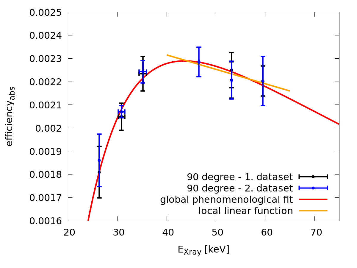
Laszlo | Calibration | efficiency values | | I have calculated the efficiency values by putting the energies of the K-REC peaks into the phenomenological (empirical) function and into the linear function (see below). The K-REC peak's position I got from a Gaussian-fit on the peak. There are 5 data sets in total:
With 1. E-calibration parameters:
-124Xe low rate measurement
-118Te 1. data set (before cable-swap)
With 2. E-calibration parameters:
-118Te 2. data set (after cable-swap)
-124Xe with scraper
-124Xe without scraper
When using the 1. E-calibration parameters, the obtained K-REC energies were much offset (124Xe_lowRate E_KREC=4.00577e+01keV, 118Te_1dataset: E_KREC=3.70922e+01keV), even though I tried all possible linear combinations of the parameters for 90° and 145°. Therefore, at the end I used the theoretical energies of the K-REC peaks from Thomas's website: http://www-ap.gsi.de/Thomas/ap_html_research/energy/index.php
Most probably, the problem is not with the 1. E-calibration itself (the source measurement looks consistent), but with the changing gate width during these measurements. These problematic data sets I marked with a " * " in the tables.
90°:
|
| 124Xe_wScraper | 124Xe_woScraper | 118Te_wScraper_part1 | 118Te_wScraper_part2 | 124Xe_wScraper_lowRate
| | K-REC E [keV] | 4,6093E+01 | 4,6116E+01 | *4,3241E+01 | 4,3135E+01 | *4,6336E+01
| | g(E_KREC) (phenomenology) | 0,002285 | 0,002285 | *0,002289 | 0,002289 | *0,002284
| | l(E_KREC) (linear) | 0,002277 | 0,002277 | *0,002295 | 0,002296 | *0,002276
| | diff. betw. f(E_KREC) and g(E_KREC) | 0,35% | 0,35% | 0,26% | 0,29% | 0,38%
|
145°:
|
| 124Xe_wScraper | 124Xe_woScraper
| | K-REC E [keV] | 4,1292E+01 | 4,1275E+01
| | g(E_KREC) (phenomenology) | 0,000736 | 0,000736
| | l(E_KREC) (linear) | 0,000750 | 0,000750
| | diff. betw. f(E_KREC) and g(E_KREC) | 1,82% | 1,83%
|
35°:
|
| 124Xe_wScraper | 124Xe_woScraper
| | K-REC E [keV] | 5,2309E+01 | 5,2478E+01
| | g(E_KREC) (phenomenology) | 0,0000532 | 0,0000532
| | l(E_KREC) (linear) | 0,0000533 | 0,0000533
| | diff. betw. f(E_KREC) and g(E_KREC) | 0,15% | 0,13%
|
> I have made also the inverse square law fits. We have data only for 90degre with the 241Am source, but both for the 1. and 2. calibrations. The 1. and 2. calibration data sets treated separate.
> 2 peaks were investigated, 59.5keV and 26.3keV, at two distances 184.8mm and 217.3mm. These distances are the sum of 4 distances:
> a = width of plastic head. uncert.: +/- 0.05mm, measured with caliper.
> b = width of the brass collimator. uncert.: +/- 0.05mm, measured with caliper.
> c = width of protector plastic ring. uncert.: +/- 0.05mm, measured with caliper.
> d= distance of the paper head. uncert: +/- 0.5mm, judged by the eye 
>
> The Be window and the dead layer of the Ge detector is not taken into account.
>
> The distances calculated as D=a+b+c+d.
>
> The conclusion is that the uncertainty coming from the distance measurements are negligible compared to the other uncertainties. The data obey the inverse square law.
>
>
> > For all 3 detector the calibration data sets were combined to include the systematics in the fit results directly. Combining means not a weighted average, just simple all data points were included into the fit --> doubled efficiency value for most of the energies.
> > The g(x) = a * (1-exp(-(x-c)/b)) * exp(-x/d) function was used to describe the behavior of the Germanium detectors for the whole range of energies (global behavior). From these fits the 80keV outlier point was excluded. This is very strange that it doesn't follow the trend, it would be nice to find out why not.
> > Between 40-75keV a linear fit was carried out as well. This can also approximate quite well this local energy range, what we need for the K-REC peaks.
> > l(x) = m*x+e
> >
> > All the fits were done by gnuplot, but it was also confirmed that ROOT gives us the same parameters + errors + chisquare. One just need to choose well the starting values 
> >
> >
> > 90° fits:
> > degrees of freedom (FIT_NDF) : 8
> > rms of residuals (FIT_STDFIT) = sqrt(WSSR/ndf) : 0.419915
> > variance of residuals (reduced chisquare) = WSSR/ndf : 0.176329
> > p-value of the Chisq distribution (FIT_P) : 0.994094
> >
> > Final set of parameters Asymptotic Standard Error
> > ======================= ==========================
> > a = 0.00308376 +/- 0.0005144 (16.68%)
> > c = 15.6259 +/- 2.035 (13.03%)
> > b = 9.36888 +/- 3.16 (33.73%)
> > d = 177.141 +/- 84.95 (47.95%)
> >
> > degrees of freedom (FIT_NDF) : 4
> > rms of residuals (FIT_STDFIT) = sqrt(WSSR/ndf) : 0.283372
> > variance of residuals (reduced chisquare) = WSSR/ndf : 0.0802998
> > p-value of the Chisq distribution (FIT_P) : 0.988405
> >
> > Final set of parameters Asymptotic Standard Error
> > ======================= ==========================
> > m = -6.22672e-06 +/- 1.836e-06 (29.48%)
> > e = 0.00256426 +/- 9.873e-05 (3.85%)
> >
> >
> >
> > 145° fits:
> > degrees of freedom (FIT_NDF) : 6
> > rms of residuals (FIT_STDFIT) = sqrt(WSSR/ndf) : 0.379472
> > variance of residuals (reduced chisquare) = WSSR/ndf : 0.143999
> > p-value of the Chisq distribution (FIT_P) : 0.990247
> >
> > Final set of parameters Asymptotic Standard Error
> > ======================= ==========================
> > a = 0.0012346 +/- 0.0006794 (55.03%)
> > c = 11.3754 +/- 4.075 (35.82%)
> > b = 15.6961 +/- 13.2 (84.1%)
> > d = 116.084 +/- 99.83 (86%)
> >
> > degrees of freedom (FIT_NDF) : 2
> > rms of residuals (FIT_STDFIT) = sqrt(WSSR/ndf) : 0.327728
> > variance of residuals (reduced chisquare) = WSSR/ndf : 0.107405
> > p-value of the Chisq distribution (FIT_P) : 0.898161
> >
> > Final set of parameters Asymptotic Standard Error
> > ======================= ==========================
> > m = -2.39246e-06 +/- 1.278e-06 (53.42%)
> > e = 0.000848859 +/- 7.329e-05 (8.634%)
> >
> >
> >
> > 35° fit:
> > degrees of freedom (FIT_NDF) : 7
> > rms of residuals (FIT_STDFIT) = sqrt(WSSR/ndf) : 1.40676
> > variance of residuals (reduced chisquare) = WSSR/ndf : 1.97896
> > p-value of the Chisq distribution (FIT_P) : 0.0538635
> >
> > Final set of parameters Asymptotic Standard Error
> > ======================= ==========================
> > a = 0.000114396 +/- 0.0002367 (206.9%)
> > c = 14.3178 +/- 8.322 (58.13%)
> > b = 16.7454 +/- 43.21 (258%)
> > d = 79.7991 +/- 173.2 (217.1%)
> >
> > degrees of freedom (FIT_NDF) : 3
> > rms of residuals (FIT_STDFIT) = sqrt(WSSR/ndf) : 1.21233
> > variance of residuals (reduced chisquare) = WSSR/ndf : 1.46975
> > p-value of the Chisq distribution (FIT_P) : 0.220529
> >
> > Final set of parameters Asymptotic Standard Error
> > ======================= ==========================
> > m = -3.7879e-07 +/- 3.143e-07 (82.99%)
> > e = 7.31447e-05 +/- 1.788e-05 (24.45%)
> >
> >
> >
> > > For the efficiency vs E fit of the 90degree Xray detector I have used the following phenomenological funciton:
> > >
> > > f(x) = a * (1-exp(-(x-c)/b)) * exp(-x/d)
> > >
> > > Here the first exponent member is a saturation curve. This part describes the passing through of the two Be windows (chamber + before detector) and through the dead layer of Ge crystal. One needs a minimum energy to enter to the detecting Ge crystal = C parameter. b parameter = characteristic absorbtion E of these nondetecting layers.
> > > The second exponent is an exponential decrease of the detector efficiency. Photons with higher energy are less detectable by the germaniums. The d parameter is the characteristic E for hard Xray and gamma (>40keV) detectability.
> > >
> > > https://www.amptek.com/internal-products/si-pin-vs-cdte-comparison
> > >
> > > //Jan's comment: the tail of this function should more or less follow a linear trend a bit above than 40 keV.
> > >
> > >
> > > In the attachment there is an example fit for 90 degree with combined 1. and 2. (before and after beamtime) calibration datasets.
> > > I made the fit with gnuplot:
> > >
> > > degrees of freedom (FIT_NDF) : 8
> > > rms of residuals (FIT_STDFIT) = sqrt(WSSR/ndf) : 0.419915
> > > variance of residuals (reduced chisquare) = WSSR/ndf : 0.176329
> > > p-value of the Chisq distribution (FIT_P) : 0.994094
> > >
> > > Final set of parameters Asymptotic Standard Error
> > > ======================= ==========================
> > > a = 0.00308376 +/- 0.0005144 (16.68%)
> > > c = 15.6259 +/- 2.035 (13.03%)
> > > b = 9.36888 +/- 3.16 (33.73%)
> > > d = 177.141 +/- 84.95 (47.95%)
> > >
> > > Laszlo's out. |
| Attachment 1: 90degree_efficiency_combined.png
|
|
| Attachment 2: 90degree_efficiency_combined.ps
|

|
|
280
|
Thu Apr 30 22:55:45 2020 |
Laszlo | Calibration | inverse square law test | | I have made also the inverse square law fits. We have data only for 90degre with the 241Am source, but both for the 1. and 2. calibrations. The 1. and 2. calibration data sets treated separate.
2 peaks were investigated, 59.5keV and 26.3keV, at two distances 184.8mm and 217.3mm. These distances are the sum of 4 distances:
a = width of plastic head. uncert.: +/- 0.05mm, measured with caliper.
b = width of the brass collimator. uncert.: +/- 0.05mm, measured with caliper.
c = width of protector plastic ring. uncert.: +/- 0.05mm, measured with caliper.
d= distance of the paper head. uncert: +/- 0.5mm, judged by the eye :)
The Be window and the dead layer of the Ge detector is not taken into account.
The distances calculated as D=a+b+c+d.
The conclusion is that the uncertainty coming from the distance measurements are negligible compared to the other uncertainties. The data obey the inverse square law.
> For all 3 detector the calibration data sets were combined to include the systematics in the fit results directly. Combining means not a weighted average, just simple all data points were included into the fit --> doubled efficiency value for most of the energies.
> The g(x) = a * (1-exp(-(x-c)/b)) * exp(-x/d) function was used to describe the behavior of the Germanium detectors for the whole range of energies (global behavior). From these fits the 80keV outlier point was excluded. This is very strange that it doesn't follow the trend, it would be nice to find out why not.
> Between 40-75keV a linear fit was carried out as well. This can also approximate quite well this local energy range, what we need for the K-REC peaks.
> l(x) = m*x+e
>
> All the fits were done by gnuplot, but it was also confirmed that ROOT gives us the same parameters + errors + chisquare. One just need to choose well the starting values :)
>
>
> 90° fits:
> degrees of freedom (FIT_NDF) : 8
> rms of residuals (FIT_STDFIT) = sqrt(WSSR/ndf) : 0.419915
> variance of residuals (reduced chisquare) = WSSR/ndf : 0.176329
> p-value of the Chisq distribution (FIT_P) : 0.994094
>
> Final set of parameters Asymptotic Standard Error
> ======================= ==========================
> a = 0.00308376 +/- 0.0005144 (16.68%)
> c = 15.6259 +/- 2.035 (13.03%)
> b = 9.36888 +/- 3.16 (33.73%)
> d = 177.141 +/- 84.95 (47.95%)
>
> degrees of freedom (FIT_NDF) : 4
> rms of residuals (FIT_STDFIT) = sqrt(WSSR/ndf) : 0.283372
> variance of residuals (reduced chisquare) = WSSR/ndf : 0.0802998
> p-value of the Chisq distribution (FIT_P) : 0.988405
>
> Final set of parameters Asymptotic Standard Error
> ======================= ==========================
> m = -6.22672e-06 +/- 1.836e-06 (29.48%)
> e = 0.00256426 +/- 9.873e-05 (3.85%)
>
>
>
> 145° fits:
> degrees of freedom (FIT_NDF) : 6
> rms of residuals (FIT_STDFIT) = sqrt(WSSR/ndf) : 0.379472
> variance of residuals (reduced chisquare) = WSSR/ndf : 0.143999
> p-value of the Chisq distribution (FIT_P) : 0.990247
>
> Final set of parameters Asymptotic Standard Error
> ======================= ==========================
> a = 0.0012346 +/- 0.0006794 (55.03%)
> c = 11.3754 +/- 4.075 (35.82%)
> b = 15.6961 +/- 13.2 (84.1%)
> d = 116.084 +/- 99.83 (86%)
>
> degrees of freedom (FIT_NDF) : 2
> rms of residuals (FIT_STDFIT) = sqrt(WSSR/ndf) : 0.327728
> variance of residuals (reduced chisquare) = WSSR/ndf : 0.107405
> p-value of the Chisq distribution (FIT_P) : 0.898161
>
> Final set of parameters Asymptotic Standard Error
> ======================= ==========================
> m = -2.39246e-06 +/- 1.278e-06 (53.42%)
> e = 0.000848859 +/- 7.329e-05 (8.634%)
>
>
>
> 35° fit:
> degrees of freedom (FIT_NDF) : 7
> rms of residuals (FIT_STDFIT) = sqrt(WSSR/ndf) : 1.40676
> variance of residuals (reduced chisquare) = WSSR/ndf : 1.97896
> p-value of the Chisq distribution (FIT_P) : 0.0538635
>
> Final set of parameters Asymptotic Standard Error
> ======================= ==========================
> a = 0.000114396 +/- 0.0002367 (206.9%)
> c = 14.3178 +/- 8.322 (58.13%)
> b = 16.7454 +/- 43.21 (258%)
> d = 79.7991 +/- 173.2 (217.1%)
>
> degrees of freedom (FIT_NDF) : 3
> rms of residuals (FIT_STDFIT) = sqrt(WSSR/ndf) : 1.21233
> variance of residuals (reduced chisquare) = WSSR/ndf : 1.46975
> p-value of the Chisq distribution (FIT_P) : 0.220529
>
> Final set of parameters Asymptotic Standard Error
> ======================= ==========================
> m = -3.7879e-07 +/- 3.143e-07 (82.99%)
> e = 7.31447e-05 +/- 1.788e-05 (24.45%)
>
>
>
> > For the efficiency vs E fit of the 90degree Xray detector I have used the following phenomenological funciton:
> >
> > f(x) = a * (1-exp(-(x-c)/b)) * exp(-x/d)
> >
> > Here the first exponent member is a saturation curve. This part describes the passing through of the two Be windows (chamber + before detector) and through the dead layer of Ge crystal. One needs a minimum energy to enter to the detecting Ge crystal = C parameter. b parameter = characteristic absorbtion E of these nondetecting layers.
> > The second exponent is an exponential decrease of the detector efficiency. Photons with higher energy are less detectable by the germaniums. The d parameter is the characteristic E for hard Xray and gamma (>40keV) detectability.
> >
> > https://www.amptek.com/internal-products/si-pin-vs-cdte-comparison
> >
> > //Jan's comment: the tail of this function should more or less follow a linear trend a bit above than 40 keV.
> >
> >
> > In the attachment there is an example fit for 90 degree with combined 1. and 2. (before and after beamtime) calibration datasets.
> > I made the fit with gnuplot:
> >
> > degrees of freedom (FIT_NDF) : 8
> > rms of residuals (FIT_STDFIT) = sqrt(WSSR/ndf) : 0.419915
> > variance of residuals (reduced chisquare) = WSSR/ndf : 0.176329
> > p-value of the Chisq distribution (FIT_P) : 0.994094
> >
> > Final set of parameters Asymptotic Standard Error
> > ======================= ==========================
> > a = 0.00308376 +/- 0.0005144 (16.68%)
> > c = 15.6259 +/- 2.035 (13.03%)
> > b = 9.36888 +/- 3.16 (33.73%)
> > d = 177.141 +/- 84.95 (47.95%)
> >
> > Laszlo's out. |
| Attachment 1: inverse_square_law.zip
|
|
279
|
Thu Apr 30 17:40:57 2020 |
Laszlo | Calibration | efficiency fits | | For all 3 detector the calibration data sets were combined to include the systematics in the fit results directly. Combining means not a weighted average, just simple all data points were included into the fit --> doubled efficiency value for most of the energies.
The g(x) = a * (1-exp(-(x-c)/b)) * exp(-x/d) function was used to describe the behavior of the Germanium detectors for the whole range of energies (global behavior). From these fits the 80keV outlier point was excluded. This is very strange that it doesn't follow the trend, it would be nice to find out why not.
Between 40-75keV a linear fit was carried out as well. This can also approximate quite well this local energy range, what we need for the K-REC peaks.
l(x) = m*x+e
All the fits were done by gnuplot, but it was also confirmed that ROOT gives us the same parameters + errors + chisquare. One just need to choose well the starting values :)
90° fits:
degrees of freedom (FIT_NDF) : 8
rms of residuals (FIT_STDFIT) = sqrt(WSSR/ndf) : 0.419915
variance of residuals (reduced chisquare) = WSSR/ndf : 0.176329
p-value of the Chisq distribution (FIT_P) : 0.994094
Final set of parameters Asymptotic Standard Error
======================= ==========================
a = 0.00308376 +/- 0.0005144 (16.68%)
c = 15.6259 +/- 2.035 (13.03%)
b = 9.36888 +/- 3.16 (33.73%)
d = 177.141 +/- 84.95 (47.95%)
degrees of freedom (FIT_NDF) : 4
rms of residuals (FIT_STDFIT) = sqrt(WSSR/ndf) : 0.283372
variance of residuals (reduced chisquare) = WSSR/ndf : 0.0802998
p-value of the Chisq distribution (FIT_P) : 0.988405
Final set of parameters Asymptotic Standard Error
======================= ==========================
m = -6.22672e-06 +/- 1.836e-06 (29.48%)
e = 0.00256426 +/- 9.873e-05 (3.85%)
145° fits:
degrees of freedom (FIT_NDF) : 6
rms of residuals (FIT_STDFIT) = sqrt(WSSR/ndf) : 0.379472
variance of residuals (reduced chisquare) = WSSR/ndf : 0.143999
p-value of the Chisq distribution (FIT_P) : 0.990247
Final set of parameters Asymptotic Standard Error
======================= ==========================
a = 0.0012346 +/- 0.0006794 (55.03%)
c = 11.3754 +/- 4.075 (35.82%)
b = 15.6961 +/- 13.2 (84.1%)
d = 116.084 +/- 99.83 (86%)
degrees of freedom (FIT_NDF) : 2
rms of residuals (FIT_STDFIT) = sqrt(WSSR/ndf) : 0.327728
variance of residuals (reduced chisquare) = WSSR/ndf : 0.107405
p-value of the Chisq distribution (FIT_P) : 0.898161
Final set of parameters Asymptotic Standard Error
======================= ==========================
m = -2.39246e-06 +/- 1.278e-06 (53.42%)
e = 0.000848859 +/- 7.329e-05 (8.634%)
35° fit:
degrees of freedom (FIT_NDF) : 7
rms of residuals (FIT_STDFIT) = sqrt(WSSR/ndf) : 1.40676
variance of residuals (reduced chisquare) = WSSR/ndf : 1.97896
p-value of the Chisq distribution (FIT_P) : 0.0538635
Final set of parameters Asymptotic Standard Error
======================= ==========================
a = 0.000114396 +/- 0.0002367 (206.9%)
c = 14.3178 +/- 8.322 (58.13%)
b = 16.7454 +/- 43.21 (258%)
d = 79.7991 +/- 173.2 (217.1%)
degrees of freedom (FIT_NDF) : 3
rms of residuals (FIT_STDFIT) = sqrt(WSSR/ndf) : 1.21233
variance of residuals (reduced chisquare) = WSSR/ndf : 1.46975
p-value of the Chisq distribution (FIT_P) : 0.220529
Final set of parameters Asymptotic Standard Error
======================= ==========================
m = -3.7879e-07 +/- 3.143e-07 (82.99%)
e = 7.31447e-05 +/- 1.788e-05 (24.45%)
> For the efficiency vs E fit of the 90degree Xray detector I have used the following phenomenological funciton:
>
> f(x) = a * (1-exp(-(x-c)/b)) * exp(-x/d)
>
> Here the first exponent member is a saturation curve. This part describes the passing through of the two Be windows (chamber + before detector) and through the dead layer of Ge crystal. One needs a minimum energy to enter to the detecting Ge crystal = C parameter. b parameter = characteristic absorbtion E of these nondetecting layers.
> The second exponent is an exponential decrease of the detector efficiency. Photons with higher energy are less detectable by the germaniums. The d parameter is the characteristic E for hard Xray and gamma (>40keV) detectability.
>
> https://www.amptek.com/internal-products/si-pin-vs-cdte-comparison
>
> //Jan's comment: the tail of this function should more or less follow a linear trend a bit above than 40 keV.
>
>
> In the attachment there is an example fit for 90 degree with combined 1. and 2. (before and after beamtime) calibration datasets.
> I made the fit with gnuplot:
>
> degrees of freedom (FIT_NDF) : 8
> rms of residuals (FIT_STDFIT) = sqrt(WSSR/ndf) : 0.419915
> variance of residuals (reduced chisquare) = WSSR/ndf : 0.176329
> p-value of the Chisq distribution (FIT_P) : 0.994094
>
> Final set of parameters Asymptotic Standard Error
> ======================= ==========================
> a = 0.00308376 +/- 0.0005144 (16.68%)
> c = 15.6259 +/- 2.035 (13.03%)
> b = 9.36888 +/- 3.16 (33.73%)
> d = 177.141 +/- 84.95 (47.95%)
>
> Laszlo's out. |
| Attachment 1: 90degree_efficiency.zip
|
| Attachment 2: 145degree_efficiency.zip
|
| Attachment 3: 35degree_efficiency.zip
|
|
278
|
Wed Apr 29 16:06:28 2020 |
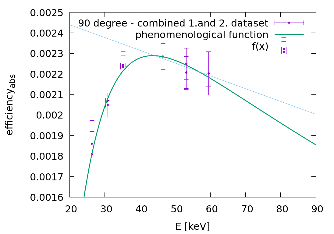
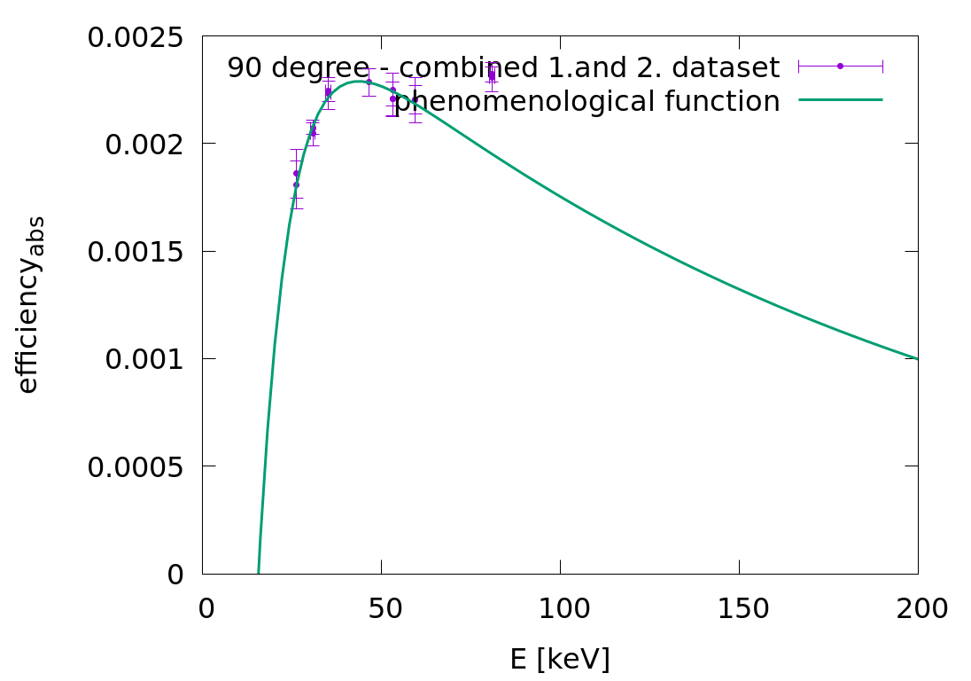
Laszlo | Calibration | efficiency fit - 90degree, combined dataset | | For the efficiency vs E fit of the 90degree Xray detector I have used the following phenomenological funciton:
f(x) = a * (1-exp(-(x-c)/b)) * exp(-x/d)
Here the first exponent member is a saturation curve. This part describes the passing through of the two Be windows (chamber + before detector) and through the dead layer of Ge crystal. One needs a minimum energy to enter to the detecting Ge crystal = C parameter. b parameter = characteristic absorbtion E of these nondetecting layers.
The second exponent is an exponential decrease of the detector efficiency. Photons with higher energy are less detectable by the germaniums. The d parameter is the characteristic E for hard Xray and gamma (>40keV) detectability.
https://www.amptek.com/internal-products/si-pin-vs-cdte-comparison
//Jan's comment: the tail of this function should more or less follow a linear trend a bit above than 40 keV.
In the attachment there is an example fit for 90 degree with combined 1. and 2. (before and after beamtime) calibration datasets.
I made the fit with gnuplot:
degrees of freedom (FIT_NDF) : 8
rms of residuals (FIT_STDFIT) = sqrt(WSSR/ndf) : 0.419915
variance of residuals (reduced chisquare) = WSSR/ndf : 0.176329
p-value of the Chisq distribution (FIT_P) : 0.994094
Final set of parameters Asymptotic Standard Error
======================= ==========================
a = 0.00308376 +/- 0.0005144 (16.68%)
c = 15.6259 +/- 2.035 (13.03%)
b = 9.36888 +/- 3.16 (33.73%)
d = 177.141 +/- 84.95 (47.95%)
Laszlo's out. |
| Attachment 1: efficiency_90degree-1an2datasets_phen_lin.png
|
|
| Attachment 2: efficiency_90degree-1an2datasets_phen_lin_bigRange.png
|
|
|
277
|
Thu Apr 23 19:09:58 2020 |
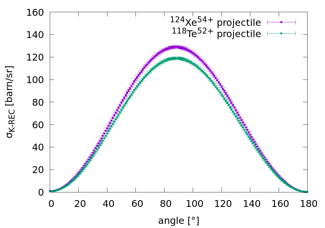
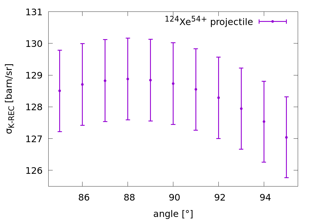
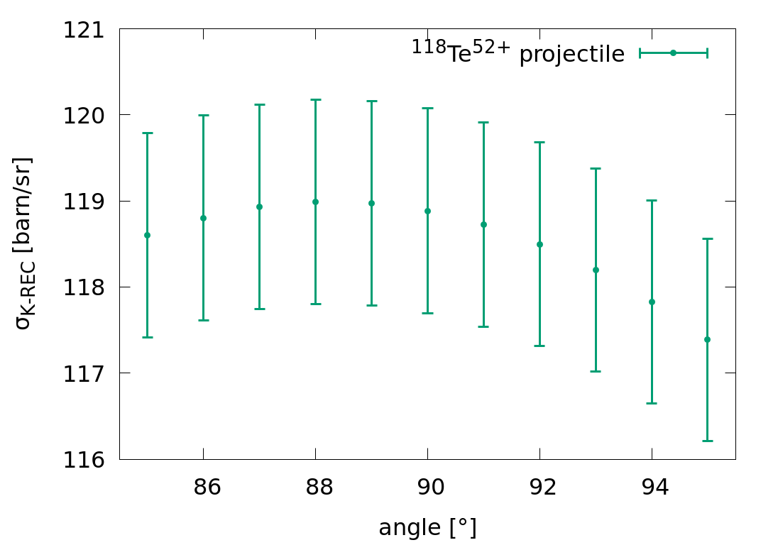
Laszlo | Calibration | theoretical K-REC cross sections | | Find attached Andrey Surzhykov's calculations for the theta angle in respect to the beam direction (in lab. frame) vs. cross section for 124Xe54+ and 118Te52+.
The calculations made for collision with two H atoms with the accuracy of 1%. There are no molecular corrections done, but these corrections are within 1%.
The photon-emission is symmetrical in the azimuthal phi angle, but asymetric in theta. The K-REC cross section is given for each integer theta angle. The problem is that our 90° and 145° xray detectors cover more integer theta-angles --> The disk shaped entrance window of the Xray-detectors is sliced for each covered theta angles, and the CS values are averaged together with the weights of the area of the corresponding slice. The 35° det had a non-disk shaped slit collimator! Was it aligned vertical or horizontal or random? I assumed that it had a vertical position --> only cs at theta=35° needs to taken into account
|
| 90° | 145° | 35°
| | weighted cs_Xe [barn/sr] | 128,444 | 41,967 | 45,550
| | weighted cs_Te [barn/sr] | 118,616 | 38,918 | 41,740
|
For the steradian values I calculated the area of the entrance window of the Xray detectors and I divided it with the area of the sphere with radius = distance between source and det. If r=radius of the entrance window, D=distance between source and det.: covered steradian = r^2*pi/(4*pi*D^2) [%], covered steradian = 4Pi*[r^2*pi/(4*pi*D^2)] [4pi]. This is valid for the 90° and 145° Xray detectors. The area of 35° det. was calculated individually.
|
| 90° | 145° | 35°
| | sr [%] | 0,00237 | 0,00076 | 0,00002
| | sr [4pi] | 0,0298 | 0,0096 | 0,00030
|
I converted barn/sr to barn in the following way: steradian[4pi]*weigthed_cs [barn/sr] = weigthed_cs [barn]. I am not 100% sure if I need here the steradian in [4pi] or in [%].
|
| 90° | 145° | 35°
| | weighted cs_Xe [barn] | 3,8247 | 0,4012 | 0,0137
| | weighted cs_Te [barn] | 3,5321 | 0,3720 | 0,0125
|
|
| Attachment 1: CS_theory_all.png
|
|
| Attachment 2: CS_theory_all.ps
|

|
| Attachment 3: CS_theory_90Xe.png
|
|
| Attachment 4: CS_theory_90Xe.ps
|

|
| Attachment 5: CS_theory_90Te.png
|
|
| Attachment 6: CS_theory_90Te.ps
|

|
| Attachment 7: DCS_Z_54_Tp_10MeV.dat
|
0. 0.8764393262751978
1. 0.9184409606576515
2. 1.0443879628122903
3. 1.2541067241116186
4. 1.5473082111252325
5. 1.9235884362763038
6. 2.3824291152290664
7. 2.9231985094824493
8. 3.5451524522204467
9. 4.2474355550499725
10. 5.029082592847121
11. 5.889020063533556
12. 6.826067919219877
13. 7.83894146477025
14. 8.926253419493086
15. 10.086516137307964
16. 11.318143980418107
17. 12.619455841203488
18. 13.988677806759991
19. 15.423945960238417
20. 16.92330931288666
21. 18.484732860465083
22. 20.106100757502197
23. 21.785219602666896
24. 23.51982182837228
25. 25.307569187584907
26. 27.146056330695448
27. 29.03281446521163
28. 30.965315090961862
29.000000000000004 32.94097380344995
30. 34.95715415797087
31. 37.011171587095994
32. 39.100297364149334
33. 41.2217626053315
34. 43.37276230320916
35. 45.55045938435645
36. 47.75198878403283
37. 49.97446153088989
38. 52.21496883482496
39.00000000000001 54.470586171241614
40. 56.7383773551312
41. 59.01539859855422
42. 61.29870254528142
43.00000000000001 63.58534227653866
44. 65.87237528199884
45. 68.15686739036538
46. 70.43589665410244
47.00000000000001 72.70655718308338
48. 74.96596292214365
49. 77.2112513677509
50. 79.43958721922418
51. 81.64816596016036
52. 83.83421736595126
53. 85.99500893349557
54. 88.1278492294348
55.00000000000001 90.23009115346127
56. 92.29913511346422
57. 94.33243210949429
58.00000000000001 96.32748672373847
59. 98.28186001390355
60. 100.19317230761206
61. 102.05910589560905
62. 103.87740762177793
63.00000000000001 105.64589136814853
64. 107.36244043326852
65.00000000000001 109.0250098024874
66. 110.63162830887903
67.00000000000001 112.18040068369685
68. 113.6695094954226
69.00000000000001 115.09721697662884
70. 116.46186673802805
71. 117.76188536923578
72. 118.99578392591334
73.00000000000001 120.16215930310027
74. 121.25969549467807
75.00000000000001 122.28716473903538
76. 123.24342855113079
77. 124.12743864126509
78.00000000000001 124.93823772099097
79. 125.67496019669385
80. 126.33683275148397
81. 126.9231748161348
82. 127.43339892989992
83.00000000000001 127.86701099212635
84. 128.223610405669
85. 128.50289011318924
86.00000000000001 128.70463652749714
87. 128.82872935716867
88. 128.8751413287365
89.00000000000001 128.84393780681756
90. 128.7352763136031
91. 128.54940594919196
92. 128.2866667143067
93.00000000000001 127.94748873698224
94.00000000000001 127.53239140486892
95. 127.04198240483984
96. 126.47695667163981
97. 125.83809524735832
98. 125.12626405355418
99.00000000000001 124.3424125779007
100. 123.4875724772668
101. 122.56285609918638
102. 121.56945492371455
103. 120.50863792770586
104. 119.38174987359533
105.00000000000001 118.19020952479832
106. 116.93550778989012
107. 115.61920579776323
108. 114.24293290600282
109. 112.80838464475747
110.00000000000001 111.31732059842409
111. 109.77156222750445
112. 108.17299063302771
113. 106.52354426597255
114. 104.82521658415874
114.99999999999999 103.08005365911461
116.00000000000001 101.29015173546108
117. 99.45765474538705
118. 97.58475178082271
119. 95.67367452595023
120. 93.72669465271724
121.00000000000001 91.746121182048
122. 89.73429781347248
123.00000000000001 87.69360022591539
124. 85.62643335241032
125. 83.53522863152084
126.00000000000001 81.42244123826835
127.00000000000003 79.29054729738027
128. 77.14204108168238
129. 74.97943219846945
130.00000000000003 72.80524276669398
131. 70.62200458781662
132. 68.43225631316218
133. 66.23854061062511
134.00000000000003 64.04340133356263
135. 61.84938069470726
136. 59.65901644792196
137. 57.474839080607154
138.00000000000003 55.29936901955791
139. 53.13511385304818
140. 50.984565571903104
141. 48.85019783229762
142. 46.73446324299586
143. 44.63979067971726
144. 42.56858262929029
145.00000000000003 40.523212566222384
146.00000000000003 38.50602236427895
147. 36.51931974563394
148. 34.56537577011455
149. 32.64642236702124
150.00000000000003 30.76464991196859
151. 28.92220485114267
152. 27.121187375328226
153. 25.363649146012833
154. 23.65159107582154
155. 21.986961165486573
156.00000000000003 20.371652399503976
157. 18.80750070256989
158. 17.296282958834453
159. 15.839715095951185
160. 14.439450235837072
161.00000000000003 13.097076913995858
162. 11.81411736919071
163. 10.592025905185897
164. 9.432187326207346
165. 8.335915447699179
166.00000000000003 7.30445168388348
166.99999999999997 6.338963713551622
168. 5.440544225441671
169. 4.610209744476686
170. 3.848899540058887
171. 3.157474617532845
172.00000000000003 2.536716793847944
173. 1.9873278583654939
174. 1.5099288196705962
175.00000000000003 1.1050592391610732
176. 0.7731766520971258
176.99999999999997 0.514656076708857
178.00000000000003 0.32978961186464684
179. 0.21878612371563544
180. 0.1817710216397566
|
| Attachment 8: DCS_Z_52_Tp_10MeV.dat
|
0. 0.6838809884595187
1. 0.7224229853331035
2. 0.8379964473235315
3. 1.030443872137824
4. 1.2995030344282912
5. 1.64480740285091
6. 2.065886722645698
7. 2.562167762440693
8. 3.1329752236222754
9. 3.7775328102535015
10. 4.494964457174398
11. 5.284295713575055
12. 6.144455279002064
13. 7.074276688431106
14. 8.072500142735743
15. 9.13777448057661
16. 10.268659287456684
17. 11.463627137414845
18. 12.721065962577109
19. 14.039281545545448
20. 15.416500129385255
21. 16.850871139764088
22. 18.340470013614155
23. 19.88330112852013
24. 21.477300826887046
25. 23.12034052881444
26. 24.81022992749396
27. 26.54472026085621
28. 28.321507653123813
29.000000000000004 30.138236519876482
30. 31.99250303019941
31. 33.88185861947699
32. 35.803813546395155
33. 37.75584048773818
34. 39.73537816460896
35. 41.73983499375132
36. 43.76659275772978
37. 45.81301028780408
38. 47.87642715343563
39.00000000000001 49.954167352475665
40. 52.043542996208096
41. 54.14185798355203
42. 56.24641165887502
43.00000000000001 58.35450244801732
44. 60.46343146728837
45. 62.5705061003606
46. 64.67304353815759
47.00000000000001 66.76837427700832
48. 68.85384557051732
49. 70.92682483078326
50. 72.98470297478
51. 75.02489771189985
52. 77.0448567688431
53. 79.0420610482222
54. 81.01402771743378
55.00000000000001 82.95831322453394
56. 84.87251623803525
57. 86.75428050772088
58.00000000000001 88.6012976437524
59. 90.4113098115192
60. 92.18211233985382
61. 93.91155624040339
62. 95.59755063611817
63.00000000000001 97.23806509697859
64. 98.8311318812456
65.00000000000001 100.37484808067475
66. 101.86737766828935
67.00000000000001 103.30695344745868
68. 104.69187890117422
69.00000000000001 106.02052994056153
70. 107.29135655180244
71. 108.5028843407837
72. 109.65371597491449
73.00000000000001 110.74253252168937
74. 111.76809468369437
75.00000000000001 112.72924392987584
76. 113.62490352300958
77. 114.454079443417
78.00000000000001 115.21586120908894
79. 115.90942259247545
80. 116.53402223430722
81. 117.08900415490466
82. 117.57379816352693
83.00000000000001 117.98792016639949
84. 118.33097237414394
85. 118.60264340941445
86.00000000000001 118.80270831562267
87. 118.93102846770623
88. 118.98755138596732
89.00000000000001 118.97231045407382
90. 118.88542454238262
91. 118.72709753780394
92. 118.49761778148746
93.00000000000001 118.1973574156676
94.00000000000001 117.8267716410606
95. 117.38639788626082
96. 116.87685489063509
97. 116.29884170226605
98. 115.65313659254451
99.00000000000001 114.9405958890601
100. 114.16215272848856
101. 113.3188157312197
102. 112.41166759952044
103. 111.44186364106933
104. 110.41063021974982
105.00000000000001 109.31926313563206
106. 108.16912593611966
107. 106.96164816028295
108. 105.69832351844508
109. 104.3807080091302
110.00000000000001 103.01041797552814
111. 101.58912810367194
112. 100.11856936456695
113. 98.60052690255144
114. 97.03683787220862
114.99999999999999 95.42938922619064
116.00000000000001 93.78011545634986
117. 92.0909962906127
118. 90.36405434806198
119. 88.60135275473215
120. 86.80499272264713
121.00000000000001 84.97711109466407
122. 83.1198778577115
123.00000000000001 81.23549362703562
124. 79.32618710409213
125. 77.39421251073887
126.00000000000001 75.44184700240568
127.00000000000003 73.47138806293053
128. 71.48515088376489
129. 69.4854657302612
130.00000000000003 67.47467529776368
131. 65.45513206022716
132. 63.429195614092336
133. 61.3992300201446
134.00000000000003 59.36760114608176
135. 57.33667401250889
136. 55.308810145072414
137. 53.28636493543301
138.00000000000003 51.27168501376619
139. 49.26710563546159
140. 47.27494808467541
141. 45.29751709737059
142. 43.337098306456504
143. 41.39595571161337
144. 39.476329176362796
145.00000000000003 37.580431954915426
146.00000000000003 35.71044825129239
147. 33.86853081318914
148. 32.056798563011185
149. 30.277334268472416
150.00000000000003 28.532182255112247
151. 26.82334616304045
152. 25.152786750176944
153. 23.522419744211014
154. 21.934113745450986
155. 20.389688182690108
156.00000000000003 18.890911324162325
157. 17.43949834560509
158. 16.037109457394024
159. 14.685348092655238
160. 13.385759158201713
161.00000000000003 12.139827350079225
162. 10.948975535442912
163. 9.81456320242211
164. 8.737884979563095
165. 7.720169226369559
166.00000000000003 6.762576696392841
166.99999999999997 5.866199274248659
168. 5.032058787863961
169. 4.261105897183412
170. 3.554219060485478
171. 2.9122035793804977
172.00000000000003 2.335790723483083
173. 1.8256369356687627
174. 1.382323118743823
175.00000000000003 1.0063540042709131
176. 0.6981576042097696
176.99999999999997 0.45808474594681375
178.00000000000003 0.28640869119862783
179. 0.18332483918885642
180. 0.14895051440953486
|
| Attachment 9: source_vs_XrayDet_sketch.pdf
|
|
|